


What is it?
Date scaffolding is a process that you can do to help fill in gaps in your data when dates are involved. It can be utilised to help with calculations or also round out your analysis. It’s typically done with datasets that contain 2 dates, typically start and end dates, providing a row for each day in between the two dates. With this, you’re able to look between the two dates and highlight changes that occurred throughout those days, e.g. seeing how headcount changes within a company or seeing how many patients a hospital had within a specific timeframe.
How it can be done in PowerBI
We’ve found a couple methods that we like for how to scaffold in PowerBI. One method can be done solely through DAX queries, while another can be done in PowerQuery.
DAX Method
This method involves creating a date table and joining that table to your dataset that you’re wishing to scaffold. At this point, you’ll then be able to create your measures and when you throw everything into a visualization, it’ll have the scaffolded data incorporated into it.
Let’s get started:
First, lets bring our data into PowerBI and then create a date table. We can do this by going into the ‘Modelling’ tab and clicking ‘New table’. We’ll be met with the usual dropdown text input box that you get when creating a new measure, which we’ll then fill out with this particular expression.
ADDCOLUMNS (
CALENDAR (MIN('BicycleRent'[Start Date]), MAX('BicycleRent'[End Date])),
"Year", YEAR([Date]),
"Month Number", MONTH([Date]),
"Month Name", FORMAT([Date], "MMMM"),
"Quarter", "Q" & FORMAT([Date], "Q"),
"Weekday", WEEKDAY([Date], 2),
"Weekday Name", FORMAT([Date], "dddd")
)
This expression uses the Start and End dates from the dataset that we’re using in this example, but you can replace those areas of the expression with the Start and End dates from the dataset that you’re using. With that information, it’s creating a calendar and set of dates and date parts based on the columns that we’re asking to be added, but using the context of the two date columns that we have to set the lower and upper boundaries of the calendar. Once this table has been created, we’ll then go to the ‘Table tools’ tab and mark this table as the date table.
After this, we’ll then create another new table, following the steps mentioned to create a date table, but this time with the following expression:
ADDCOLUMNS (
FILTER (
CROSSJOIN (
'BicycleRent',
CALENDAR (MIN('BicycleRent'[Start Date]), MAX('BicycleRent'[End Date]))
),
[Date] >= [Start Date] && [Date] <= [End Date]
),
"Daily Rental Price", 'BicycleRent'[Price (£)] / (DATEDIFF('BicycleRent'[Start Date], 'BicycleRent'[End Date], DAY) +1)
)
What this calculation is doing is that it’s essentially joining that newly created Date table with the existing dataset that we have for Bicycle rentals, based on the date field that we have now. It’s joining so that we get rows from the Date table that fit in the specification of ‘Date >= Start Date && Date <= End Date’, meaning that we only want dates brought into the table that are greater than or equal to the start date of the rentals and where the date is less than or equal to the end date of the rentals. This is essentially the scaffolding process in play here, where we’re adding rows to the data for the dates in between those start and end dates. Alongside this, we’re adding another column to the dataset, which is the ‘Daily Rental Price’. What this part of the calculation does is that we take the total price of the rental [Price (£)] and divide that by the difference in days between the Start Date and End Date, and also adding another day to that difference in days since with rentals, the fee begins on the same day when you rent something. This will then give us the price of the rental per day.
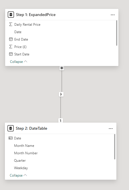
Once this has been created, we’ll go into the ‘Model view’ tab and take a look at the relationships between our tables. What we’ll be doing here is joining the ‘Date’ field within that Date table to the now existing ‘Date’ field in the newly created table that we’ve just created. This relationship will come in the form of a ‘Many to one’ relationship, with the ‘many’ coming from that newly created table that has the Daily Rental Price column that we’ve added, and the ‘one’ part of the relationship coming from the date table, as pictured below.
Once this has all been completed, you’ll be able to use the new dataset that we’ve made and throw out some visualizations that’ll now reflect your freshly scaffolded data.
PowerQuery Method
This method is instead simpler and can all be done in the PowerQuery window, before you load your data into the main PowerBI page that we’re all familiar with.
What we do here is that we find out the number of days +1 between the End Date and Start Date, and then with this number we’re able to know how many rows we need to add in to act as the scaffold. We can do this with, in the context of the Bicycle rental dataset we’ve been using, the following expression, which can be used when adding a column to the dataset. We’ll call this column ‘Duration’:
Duration.Days([End Date] – [Start Date])+1
As described in the paragraph above, this expression is finding the number of days between the End Date and the Start Date, with 1 being added to that final number since rentals start on the day of purchase, rather than the day after.
With this information now, we can pretty much go into the scaffolding process. What we’ll do is add another column to our dataset, but this time with the following expression, naming the column as ‘Date’:
List.Dates([Start Date], [Duration], #duration(1,0,0,0))
This expression broken down can be understood as being relatively similar to a DateAdd expression, where the date that you’re specifying in the expression is the ‘Start’ date. It can be seen as the starting point of where you’re adding rows of data to. The [Duration] part of the expression is the number of rows that you want added. Since in our example, that duration column has the number of days between the end date and the start date, we can use this as this part of the expression since that has the correct number of rows we’ll need added. Finally the ‘#duration’ part of the expression is how we tell it what sort of date increments we’ll be needing, e.g. days, hours or minutes. With the #duration command’s structure, we’ve put the following into the brackets for the command – 1,0,0,0. The order here is in the format of Days, Hours, Minutes and Seconds. We’ve put a 1 in the ‘Days’ section of the command as we just want an increase in 1 day for each date added, with zeroes thrown in for the other 3 options since we don’t need increases in those sections.
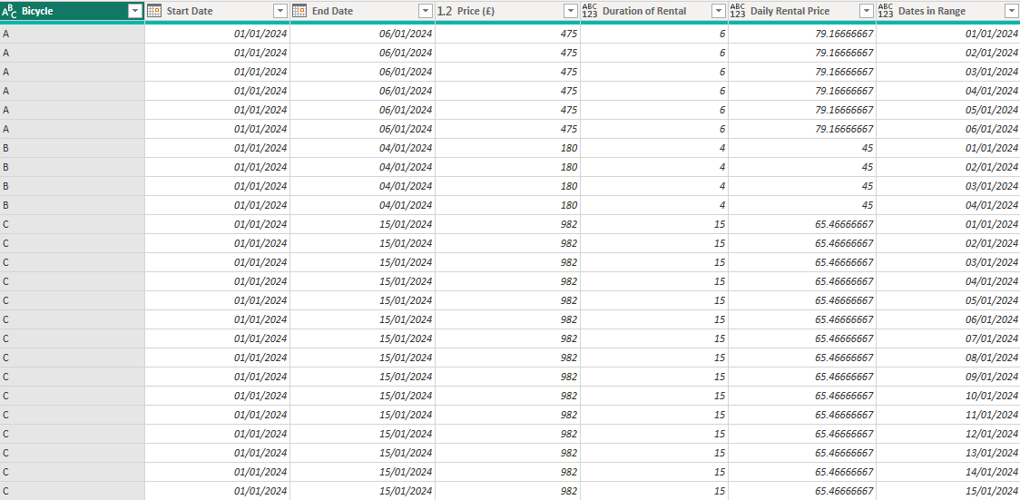
Once this column has been added to the dataset, you’ll just need to expand it out to rows and you’ll then see a familiar sight – scaffolded date data. Here’s how our data looks at the end of this process:
Hopefully this has helped with understanding a couple ways to scaffold your data in PowerBI and when you would typically go about doing it. Happy scaffolding!