


I've watched enough NWSL matches to know when a team's shape is wrong. The same instinct applies to database design and this source table needed a rethink.
My process had four stages: sketching an architecture, refining it in dbdiagram.io, ingesting the raw data into Snowflake, and transforming it with SQL.
Planning the Architecture
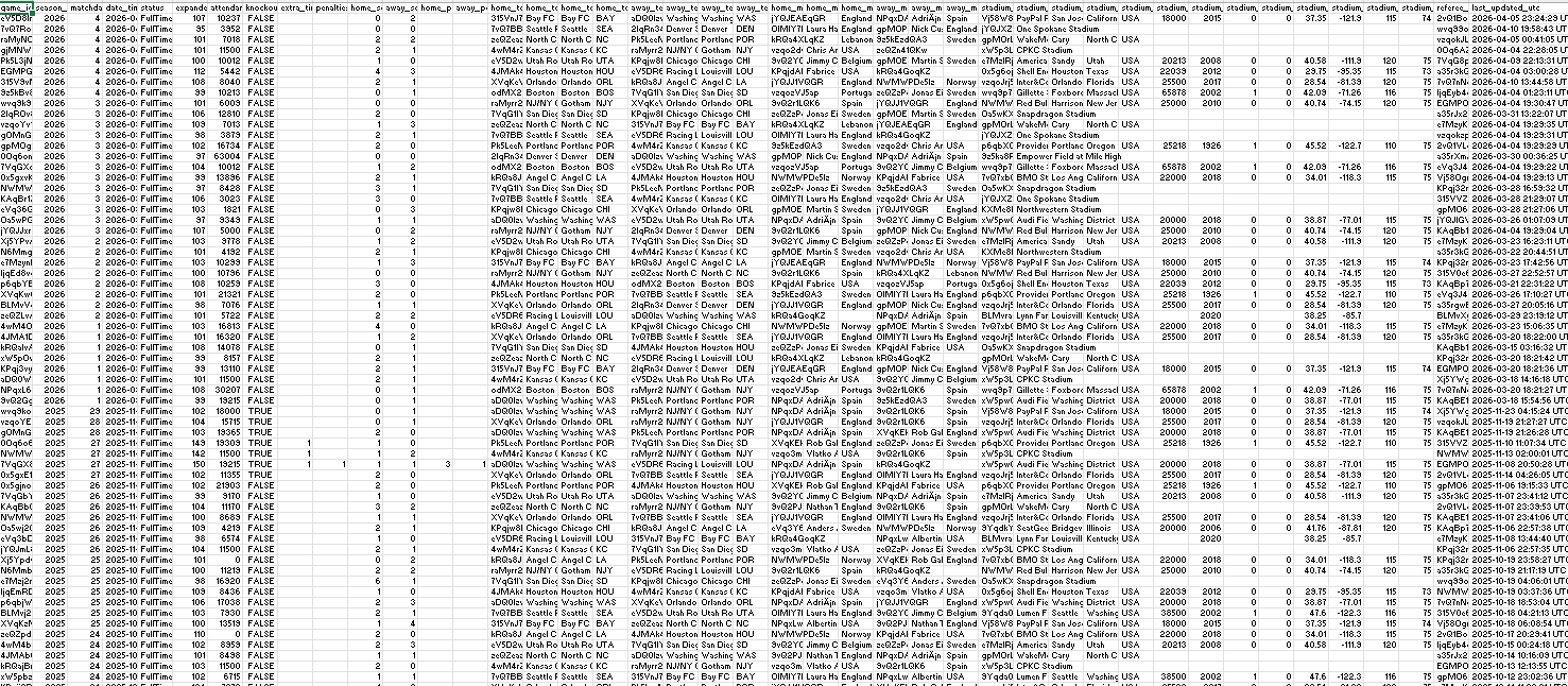
The source dataset covers every NWSL match since 2017, with home and away team info, managers, referees, and stadium details all crammed into a single wide table. Useful, but not efficient to query repeatedly.
My goal was a classic star schema: one central fact table for match results, surrounded by dimension tables for the entities that don't change game to game. This keeps the fact table lean and avoids storing repetitive strings like team names or stadium addresses on every row.
Based on what was in the data, the natural split was:
- Fact table: one row per game, with scores, dates, and foreign keys
- Dimension tables: teams, managers, referees, stadiums — each with a unique ID
I sketched this out roughly to get an initial breakdown. I also considered additional tables that were already separated that I could add such as Player goals, refs, and players.
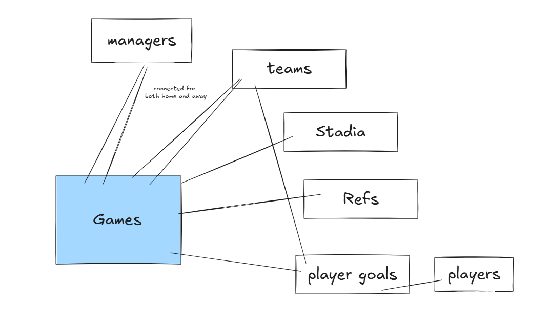
Using dbdiagram.io, which I wrote about in an earlier blog post here, I cleaned up this diagram and added additional information about the specific foreign keys and fields. This provides a clear map for anyone interested in using this data in the future.

Ingesting Data into Snowflake
Snowflake's UI makes local file uploads straightforward. In the navigation bar, the upload icon offers a few options.
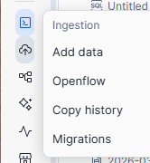
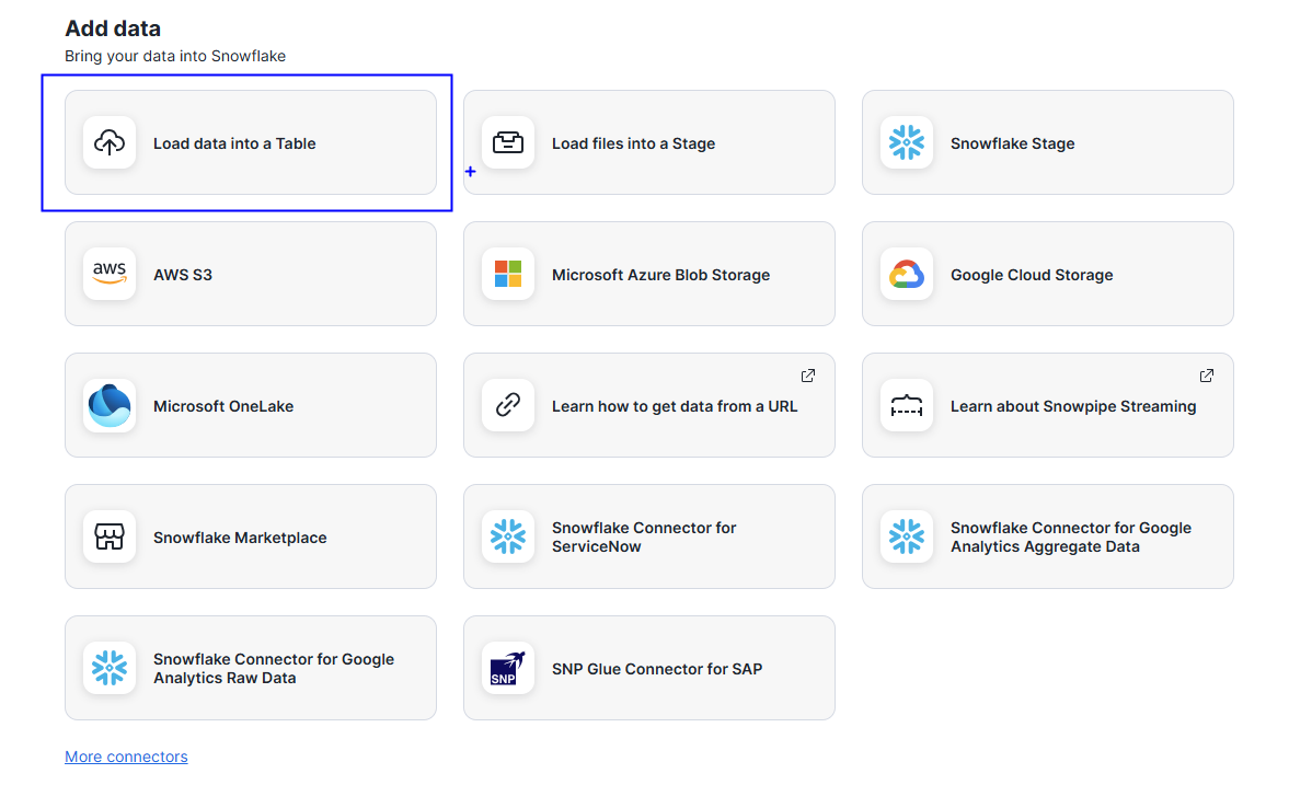
I chose Load data into Table since I was working with a local CSV.
From there I selected the target database and schema, named the new table in the popup, and Snowflake handled the rest: column detection, data types, and staging. Once complete, the table was immediately queryable in that schema.
Building the Dimension Tables
With the raw data loaded, I used SQL to create each dimension table, renaming columns for readability along the way.
The trickiest part was the teams table; because each game has both a home and away team, I needed to combine both into a single unified list of unique teams. I used a UNION to merge the two sides:
N.B. CREATE OR REPLACE will overwrite an existing table so use with consideration.
-------------------------------- TEAMS ------------------------------
CREATE OR REPLACE TABLE teams AS
SELECT DISTINCT
    home_team_id            AS team_id,
    home_team_name          AS team_name,
    home_team_short_name    AS team_short_name,
    home_team_abbreviation  AS team_abbreviation
FROM nwsl_games_wide
WHERE home_team_id IS NOT NULL

UNION

SELECT DISTINCT
    away_team_id,
    away_team_name,
    away_team_short_name,
    away_team_abbreviation
FROM nwsl_games_wide
WHERE away_team_id IS NOT NULL;
I used the same UNION pattern for managers, since they also appear in both home and away columns.
Building the Fact Table
With all the dimension tables in place, the fact table was straightforward: keep the game-level metrics and replace the repeated entity details with their corresponding IDs.
-------------------------------- GAMES (FACT TABLE) ------------------------------
CREATE OR REPLACE TABLE games AS
SELECT
    game_id,
    season_name,
    matchday,
    date_time_utc,
    status,
    attendance,
    expanded_minutes,
    knockout_game,
    extra_time,
    penalties,

    -- Scores
    home_score,
    away_score,
    home_penalties,
    away_penalties,

    -- Foreign keys to dimension tables
    home_team_id,
    away_team_id,
    stadium_id,
    referee_id,
    home_manager_id,
    away_manager_id,

    last_updated_utc
FROM nwsl_games_wide;
There are ways to break this down further, but this structure hits a good balance of simplicity and query efficiency for most analysis.
If you want to see what this data looks like in practice, check out my Gotham FC dashboard on Tableau Public: Gotham FC Game Dashboard
https://public.tableau.com/app/profile/sita.pawar/viz/GothamFCGameDashboard/FCGameDashboard
N.B. This data was initially pulled from the itscalledsoccer API. Tables were combined for the purposes of this demo/exercise.