


An step by step walk through on web scraping HTML tables using Alteryx and R Studio independently.
In this blog post, created by Markus Göhler and myself, we will walk you through an example of web scraping an HTML table, showcasing both R studio and Alteryx.
Check out the German version by Markus via this link (to be added soon).
We used the List of World Heritage in Danger wikipedia page, which is featured in the book: Automated Data Collection with R: A Practical Guide to Web Scraping and Text Mining by Simon Munzert, Christian Rubba, Peter Meißner and Dominic Nyhuis (John Wiley & Sons, Ltd 2015).
Our R Studio example closely follows the case study presented in this book. We highly recommend reading it, as it clearly explains the basics of web language/structure, data gathering from the web and using R to automate your web data collection.
How the blog is setup
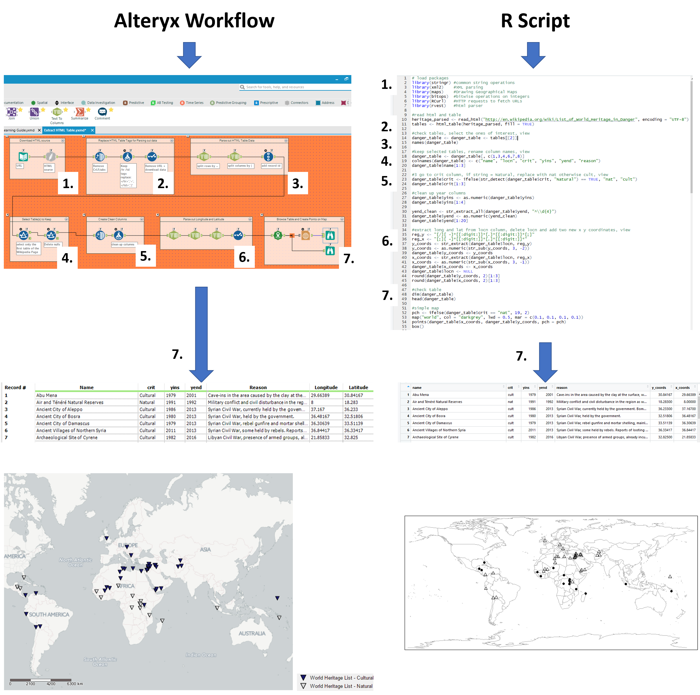
From here onwards, we split the blog up into two separate columns, the left outlining the Alteryx workflow and the right, the R script. We have divided up parts of the work into seven pieces, to try and make it easier to compare the different operations used between R and Alteryx to attain the same results.
Do note that some operations will seem long in one software over the other, however, this is simply due to the way they operate and we found that it took about the same time to do this work in both pieces of software. R Studio has some convenient packages available to shortcut the html parsing, whilst Alteryx provides handy tools to auto clean your fields and quickly parse out data.
Following the flow below, we go from downloading the data all the way to a quick visualisation. The Alteryx workflow and R script can be downloaded through a link at the end of this blog, enjoy!
1. Setting up and connecting to the data
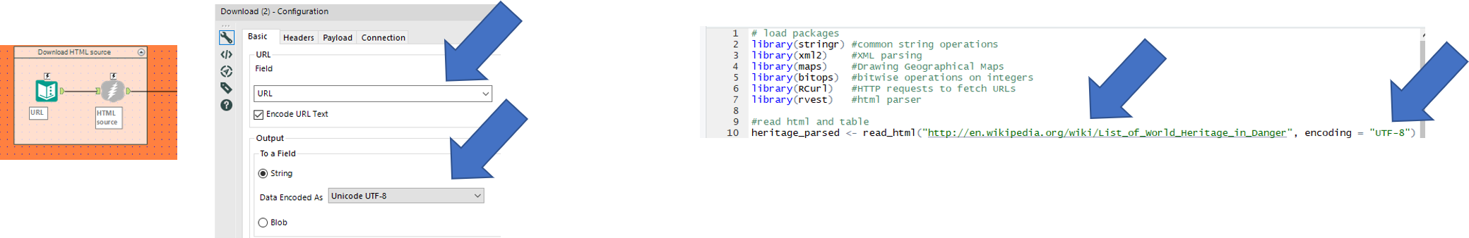
| We start with a text input file to paste in the URL of the web page and connect it to a download tool to read it in.
Make sure to set the output to a string field. This step reads in the whole HTML of the web page as a text field. |
In R, we start by loading all the packages required to carry out the operations further down.
Make sure to install the packages if you haven’t already, through the CRAN R Repository or through the packages pane in the R studio. For Alteryx users, R packages can be compared to Alteryx Macro’s, created by other users, but rather than having a bunch of settings to choose from it comes with a set of functions to call upon and apply to your data. Next, we read in the URL using the read_html function from the xml2 package |
2. Identifying HTML tables
For this example we are using the ‘’currently listed sites’’ as found on the web page.

Prior to going through the steps on how to select just this table in Alteryx and R, we will quickly show you how to inspect the HTML elements of this page using Google Chrome to better understand the steps further below.
If you are on any page in Google Chrome and you open the elements tool (Ctrl + Shift + C), a pane will show up in which you can inspect the HTML of the page.
If you hover over the lines with your mouse, it will highlight the elements in your browser, i.e. you can drill down into the HTML in order to find the Table, headers, rows and cells you are interested in.
By looking at the GIF above, we find that the <thead> elements are responsible for our table headers, whereas <tbody> contains our table info.
Furthermore, drilling further down into these elements we find that the <tr> elements contain row information, containing <td> elements for each cell.
FYI, if you want to find the end of, for instance a cell, simply look for </tr>. The forward slash implies the end.
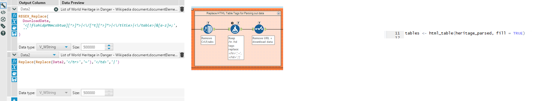
| The HTML has been imported into a single text cell, which we clean to remove tabs, linebreaks, and duplicate whitespaces with the data cleansing tool.
Next is to identify all HTML table end tags ( </tr> and </td> as described above) and replace them with characters that aren’t used in HTML in order to parse out the data with text to rows and text to columns. Using regex_replace on the downloaded data, we remove unwanted tags from </tr> and </td>, before replacing </tr> with ~ and </td> with | . (named: data2) (many thanks markp for these formulas) The select tool is used to remove the old download data field. |
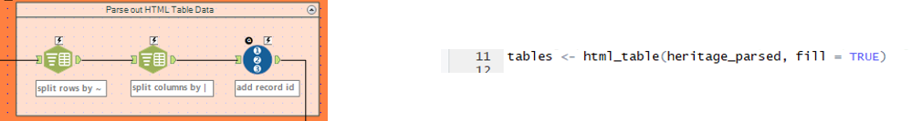
In R, we utilize the html_table function from the rvest package to read in all the HTML tables contained in the downloaded data and store it under the name: tables |
3. Parsing out the HTML tables
| Using the replaced HTML table end tags in our created data2 field, we can split to rows on ~ followed by split to columns on | (8 columns, data21-28).
We add a record id for the next filter step. |
This step is included in the previous step (2.) using the html_tables function from the rvest package |
4. Select the tables to keep
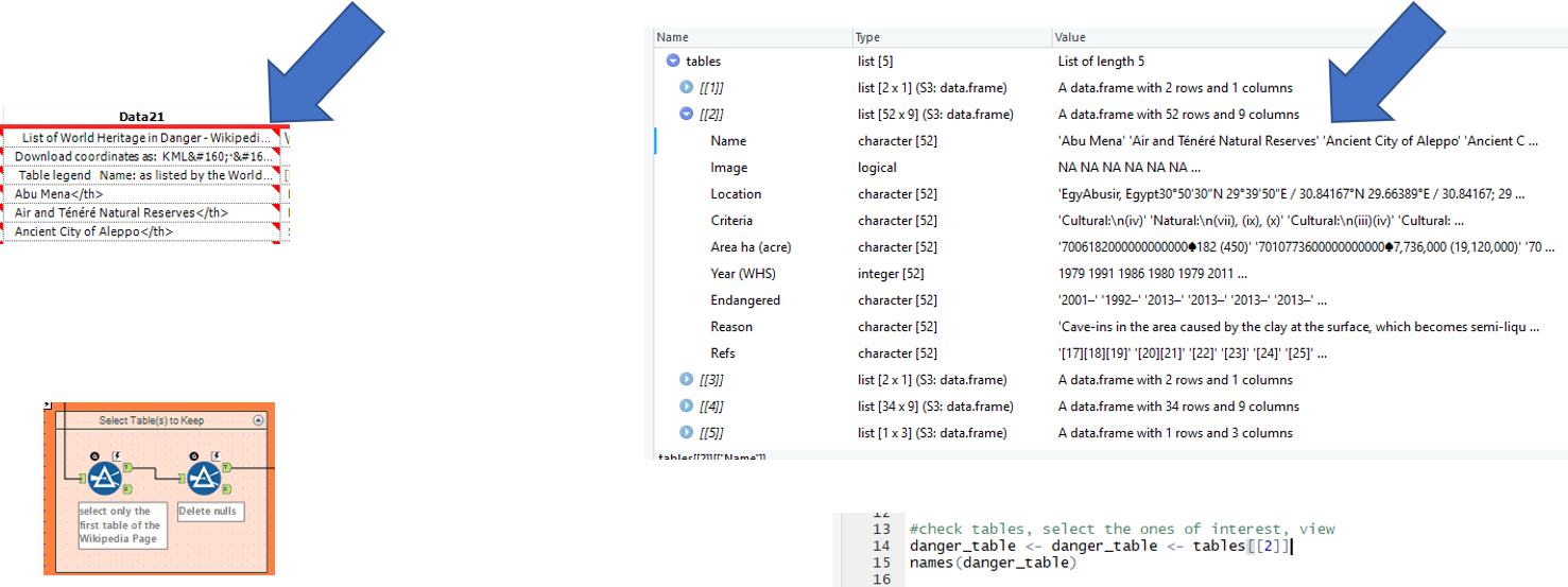
| Using the added record id we find that the the ‘’currently listed sites’’ table ends after line 57 and filter the rest out.
Further empty fields (due to a few header lines) are removed by filtering the data26 column on: Is Not Null |
Inspecting the tables imported into R, we find that Table [[2]] contains the ‘’currently listed sites’’
We further save this table under the alias danger_table and inspect the column names. |
5. Creating clean columns
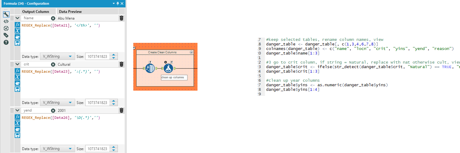
| Using the Data Cleansing tool, we replace any unwanted nulls with blanks whilst also removing white spaces, tabs, line breaks, and duplicate white space in the data 21-28 fields
Next, using a formula tool, we create the clean Name, criteria (crit) and year end (yend) fields. Regex_replace functions are used to remove: ‘</th>’ to exactly match the </th> from the Name, matching on ‘</th>’ and replacing it with nothing ‘’ ‘:(.*)’ to match the colon and everything after the criteria, replacing it with nothing ‘’ ‘\D(.*)’ t match any non-digits and everything afterwards after the yend, replacing it with nothing ‘’ |
We select only the columns of interest (1, 3, 4, 6, 7, 8) and rename them (name, locn, crit, yins, yend, reason) using the colnames function.
Upon checking the first 3 rows (danger_table$name[1:3]), we find that the criteria and year fields contain unwanted characters. These are cleaned using stringr package functions. For the criteria, we use str_detect to look for Natural and if matched, replace with ‘nat’ else ‘cult’ to remove the unwanted characters. For yins we can use the as.numeric function to remove unwanted characters from the year numbers by forcing it into a numeric field. For yend, we had to use a similar regex expression as in alteryx to first extract the last year in the field (contained start and end year prior to this), by matching ^\\d{4} (from the back of the field, search for 4 digits. Followed by the as.numeric function as above for yins. |
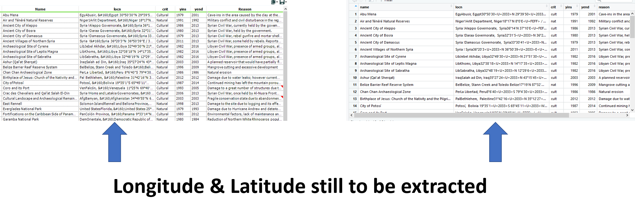
These operations leave us with a near complete table in both R and Alteryx, just missing the longitude and latitude fields!
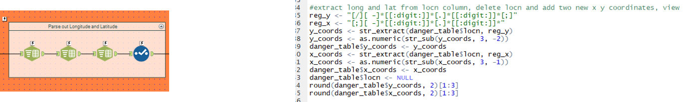
6. Extracting Longitude and Latitude
At this point, both tables contain a column containing longitude and latitude data in the format of:

Encircled in orange are the long and lat that we need to extract.
In the case of Alteryx, we used 3 text to column tools to separate out the values we we want.
A select tool is added to force the long lat’s into doubles to remove any unwanted characters, whilst at the same time remove all the unwanted fields. |
In the case of R, we define two regular expression (regex) functions to exactly match the longitude and latitude
Latitude: reg_y <- “[/][ -]*[[:digit:]]*[.]*[[:digit:]]*[;]” Longitude: reg_x <- “[;][ -]*[[:digit:]]*[.]*[[:digit:]]*” These are then used in string extract functions, stored as new field and converted to numeric fields whilst removing the old fields. |
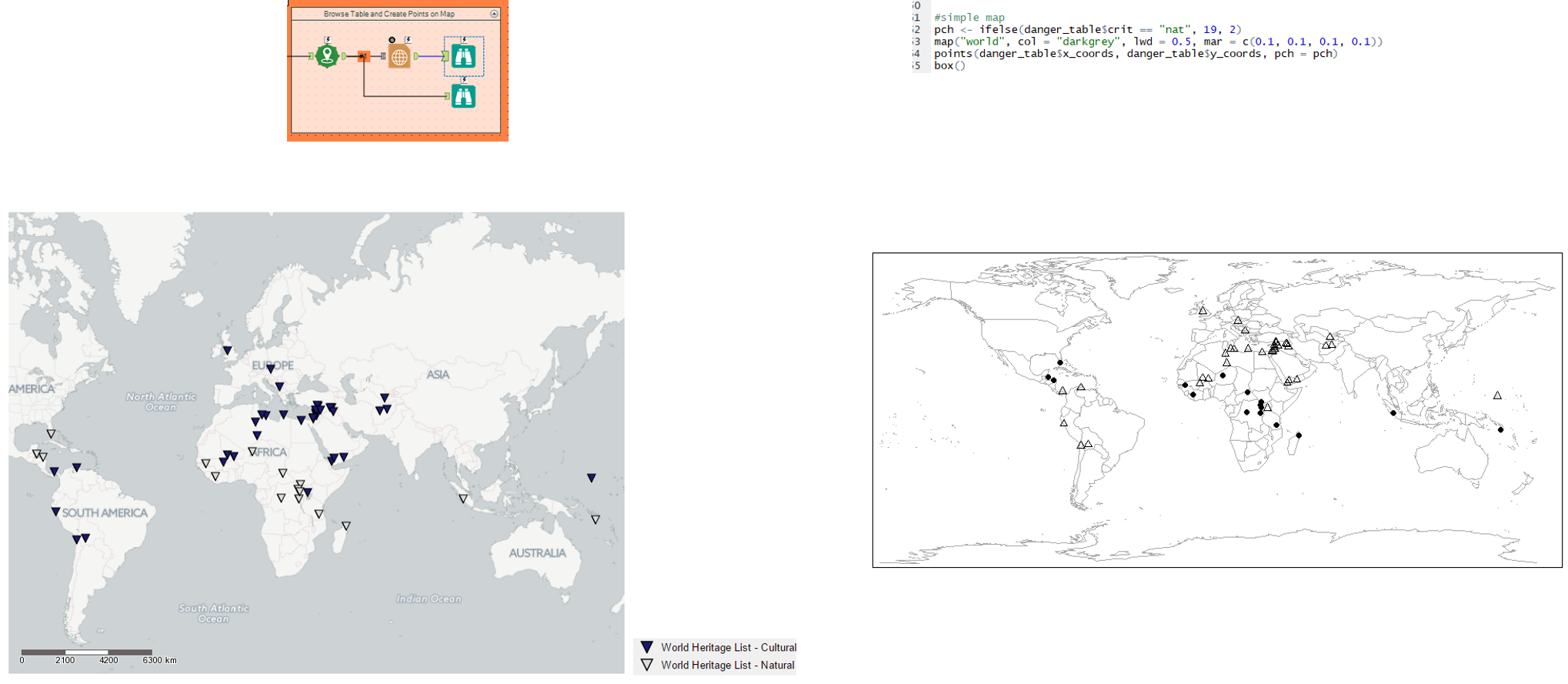
7. A quick geographical visualisation
| Using the spatial tool: create points, we create the spatial objects for each ‘currently listed site’ on the world heritage list.
The report map tool can then be used to change the colour of the symbol, based on whether the criteria is Natural or Cultural. |
We use the map package to create a map and populate it with the longitude (x_coords) and latitude (y_coords).
The lat and longs, including Natural and Cultural criteria, are labelled on the map using the points function. |
8. A quick conclusion
After showing both ways how to handle web scraping, it’s time for a little resume.
If you compare tools vs. pure code, Alteryx is going to win this battle (18 tools vs. 36 lines of R code). The next check would be the speed and this fight will go to R. Alteryx needs 2.6 sec to finish the workflow which is almost three-times slower than R (0.97 sec).
Another thing is the amount Regex used throughout the flow/script, which is higher when using Alteryx. However, it would be the same for R if we excluded pre-defined R packages. The same effect could be achieved in Alteryx by creating macros and share them on the Alteryx Gallery.
9. Download the workflow and script
Hopefully we have given you some insight into web scraping HTML tables, helping you to overcome the first step into web scraping or to further progress your knowledge.
Obviously, it will be difficult to fully grasp the workflow and script from just this blog. Therefore, you can find the alteryx workflow and R studio script in the links below for you to look at, play with and use to your advantage.
We have tried to outline what each step does to help and walk you through it.
https://data.world/robbin/web-scraping-html-tables-analteryx-workflow-and-r-script
That’s it for now. Feel free to contact us about any of the content on Linkedin or Twitter @RobbinVernooij – Markus Göhler.