


Since joining the Data School at the beginning of August as part of DS21, we have been gently introduced to the various tools we will be learning: Tableau, Tableau Prep, and Alteryx. Our first Alteryx session was on the 11th with Dan Farmer, who introduced us to the interface, some fundamentals of data management, and walked us through some of the many things that Alteryx can do.
I come from a background where I have some experience using R, and I was intrigued to see the differences and how the two matched up against each other, especially considering my immediate bias towards coding. I love using R, and was both anxious and intrigued about how a different program – Alteryx – was the preferred program of choice at TIL. Instead of being a coding language, Alteryx allows you to organize workflows for data, using icons, functions and logic to manipulate, model, and output data. There are many pre-built functions inside Alteryx, which work similarly to functions within most data manipulation languages such as R, and Python.
I decided to explore a workflow that we worked through in our introduction class, and compare how I would clean the data on different interfaces. Something I was immediately shocked with was how within 30 minutes of our class, we were able to read-in data, and perform some quite impressive cleaning and manipulating techniques to our dataset. Compared to R, which took me weeks to learn, this was one of the biggest things that stood out to me.
TL:DR This blog will document my different approaches to how I would clean, and prepare data when using different applications. The different experiences really highlight the power of Alteryx, especially with the very brief experience I have had with it.
The Data & Workflow
We will be importing a dummy dataset provided by Dan which looks at sales data from Austria between 2014-2018, which can be accessed here alongside the R script and Alteryx workflow. It is a small dataset, with only 270 rows which is a breeze for both R and Alteryx to handle. However, typically with data, it required preparing before it could be useful to us, consisting of the following steps:
- Renaming some column names such as CUSTNAME, and ensuring that upon import, data types were correctly formatted
- Adding relevant columns, such as Profit and Revenue
- Cleaning the OrderID column, which must be done by extracting the true ID number which was the final set of numbers in the column, after the country code and the year of purchase
- Furthermore on OrderID, filling in missing values that occur when multiple orders are placed on the same day by the same person
The Approach: Alteryx
The entire workflow for this process could be completed in just one work stream, using 7 separate tools.
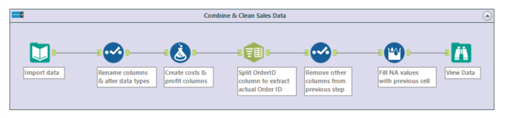
Step 1: Import the Data
Importing data into Alteryx is easy, and consists of dragging a ‘Input Data’ tool onto the canvas, and selecting from the drop-down the csv file ‘Austria.csv’. This can also be achieved by dragging the file from a browser window onto the canvas! By clicking the tool, we can immediately see a preview of the first 100 rows, and configure import parameters such as delimiters (this is not required for this tutorial).
Step 2: Rename Columns & Fix Data Types
For this step, we require the select tool, which will allow us to easy handle these fixes in just a few clicks. Firstly, we want to change the column name CUSTNAME, and change it to ‘Customer Name’, to avoid confusion and provide easier headers to work with. Next, we must change columns Sales, Quantity and Unit Cost to a numeric data type. This will allow us to do operations on the data, since Alteryx is unable to compute calculations on strings.
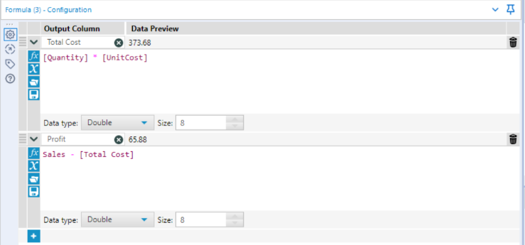
Step 3: Adding Total Costs & Profit columns
Since we are given sales and unit cost information, it would be useful to create new columns showing us both the total costs, and then profit from each transaction. This is easily done by dragging onto the canvas ‘Formula’, and entering the following into our Configuration tab:
Step 4: Extracting Order ID
The next step, when Dan mentioned it, concerned me that it was going to be a really complex task. However, with Alteryx, it requires 1, painfully easy step. In the ‘parse’ tab, simply drag a ‘text to columns’ tool onto the workspace, and connect it to our formula tool on the canvas. Next, we want to split the OrderID column into 3 separate columns, because, if we look at the first entry of the data, ES-2015-1043483, the format is as follows: COUNTRY-DATE-ORDERID. To extract the part we want (the green text), we simply use the ‘text-to-columns’ tool found within the parse tab. Dragging and connecting this to our previous step gives us the option to split our target column, Order ID, into 3 respective columns, split by the delimiter ‘-‘.
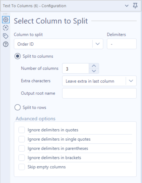
By specifying the column to split (Order ID), the delimiter (-), and the number of columns we want to split it to (3), the output gives us 3 separate columns, which are named ‘1, 2, 3’ holding the information ‘ES, 2015, 1043483’ respectively.
Step 5: Removing Unnecessary Columns Produced by Step 4
Since we created 3 columns from our previous step, but only need 1- the next job is to remove the other 2 columns, leaving us just with the true Order ID column. This can be done with another select tool, which allows us to both rename the column from ‘3’ to ‘Order ID’, and drop columns ‘1’ and ‘2’. We are now ready for the final step.
Step 6: Imputing Missing Values in Order ID
The final step in our workflow is to fill our Order ID downwards in instances that they are missing. This is a convenient problem to have, and Alteryx makes this step equally as easy to fix. Navigating to the ‘Preparation’ tab, and dragging ‘Multi-Row-Formula’ to the canvas allows us to insert a formula that allows us to fill all NAs existing within Order ID. First, select Order ID as our existing field to update, and place the following formula:
IF isnull([Order ID]) THEN [Row-1:Order ID] ELSE [Order ID] ENDIF
What happens here is, Alteryx scans down the column, and if it encounters a null value, it looks above the cell, and pastes that value into the empty cell. If the cell is not empty in the first place, it simply leaves it unchanged. This concludes our data preparation, allowing for further operations to be carried out in the future.
The Approach: R
Quick disclaimer – I have not extensively used R since 2019, and I have chosen to R without using additional packages whenever possible.
Step 1: Reading Data & Installing Packages
The first stage is to read in data, and due to the nature of R and the functionality we need, we must assign this csv file to a variable named ‘Austria’, and install the required package for later. If you are following along, you will need to provide the filepath inside the ‘read.csv’ function, or set your working directory as the folder that the data is in (tutorial here)
Austria <- read.csv('Austria.csv')
install.packages('zoo')
library('zoo')
Step 2: Renaming Columns & Fixing Data Types
Fortunately, R was able to identify our numeric classes, meaning that we do not have to change the data types for ‘Sales’, ‘Quantity’, and ‘Unit Cost’. However, we must rename the column ‘CUSTNAME’ (the 14th column in the dataset), complying with R’s requirement that we cannot have spaces between our column names.
colnames(Austria)[14] <- 'CustomerName'Step 3: Adding Total Costs & Profit Columns
Creating new columns in R is easy, and this can simply done by referencing our dataset, and create the new columns using ‘$’.
Austria$TotalCosts <- Austria$Quantity * Austria$UnitCost
Austria$Profit <- Austria$Sales - Austria$TotalCosts
Step 4: Where It Gets Confusing
Things got tricky here, and the problems with R began to become quite clear. Perhaps due to my rustiness in R, lack of knowledge of workarounds, or poor package knowledge, the next 2 stages were incredibly frustrating. In order to get the desired output, we had to switch steps 4 and 6, since the method I used to split the OrderID columns into 3 separate columns would remove all null values from the OrderID column, leaving us with only 183 rows.
Therefore, the workaround was to fill the missing NA values first, and then split the values into separate columns. This is where our ‘zoo’ package comes in, and a tedious approach follows to allow the required function to work. First, we must ensure all empty rows in OrderID are assigned ‘NA’. Then, we assign the OrderID column to a new variable (OrderID_Imputed), saved as a dataframe (or our function to fill NAs will not work), and then call our function from zoo, which carries the last observation forward for any referenced column, allowing us to yield the same result as Alteryx. After renaming the column to OrderID_Filled, we are ready to now split the column up into 3 separate columns as shown in Step 4 of the Alteryx workthrough.
OrderID_Imputed <-  as.data.frame(na.locf(Austria$Order.ID))
colnames(OrderID_Imputed)[1] <- 'OrderID_Filled'
Step 5: Splitting OrderID Into 3 Columns
Before updating our dataset with our amended OrderID column, it made sense to extract the actual Order ID first, which was a frustrating process. The aim here is the same as Step 4 in the Alteryx workflow, splitting OrderID into 3 columns, and then removing the 2 unnecessary columns, and finally attaching it back onto the main dataset. I’m sure there was an easier way, but Stack Overflow again showed me that many people struggled with this process.
OrderID_Impute_Split <- data.frame(do.call('rbind',
   strsplit(as.character(OrderID_Imputed$OrderID_Filled), '-',fixed=TRUE)))
Essentially, this function says: In the dataframe format, apply the function ‘rbind’ (binds a vector row-wise) to a split version of our Order ID data where NAs have been replaced, where new columns form every time a ‘-‘ is encountered.
Essentially, this function says (reading outwards): split the contents for each row of OrderID_Filled at ‘-‘, then bind this together in the format of a dataframe. This is because, without binding it by rows, it would come out as a vector, instead of our desired format. To finish this work off, simply adding the correct OrderID column back (the variable OrderID_Impute_Split) to the original dataset finalises this workflow. We must choose the third column from this variable, since it holds the desired Order ID.
Austria$Order.ID <- OrderID_Impute_Split$X3Summary & Reflections
I love R, and I will make every excuse to use it; but I think Alteryx quite clearly demonstrates it’s power when it comes to data cleaning. The ability to, within a few clicks, perform tasks so complex in Alteryx was a breathe of fresh air. Similarly, the endless amount of tools at your disposal with Alteryx is also very impressive. One of my favourite things about this work flow was that everything could be completed within 1 workflow stream (meaning, we did not have to separate any data and re-join it later on to complete the task within Alteryx). In R, it required us to introduce new variables, re-assign column names, and constantly track back to ensure you are using the correct variable when making a permanent change to the original dataset. Ultimately, I feel this made Alteryx less error-prone and easier to debug when encountering errors, since you can simply disconnect streams of work and amend your work as you go. Obviously both Alteryx and R have their separate strengths and weaknesses, but I can understand why here at the Information Lab, Alteryx is used as the primary data preparation tool!