


In my introductory blog on dbt, I made mention of how modularity in dbt is an asset in data transformation and sets it apart. In this blog, I seek to touch on this topic with a very simple example for a better understanding.
What is modularity?
Modularity in simple terms is the process of breaking down complex models into tiny bits with defined relations which connects these bits. Just like how a camera is built, the individual parts are built and later brought together to give us the finished product.
The importance of this methodology in data transformation cant be understated because:
- It simplifies lengthy code which aids in readability and understanding.
- Due to its simplicity, troubleshooting errors becomes a snap event.
- Due to the breakup in models, it allows model referencing which is the root of clean and understandable code.
- Code modularity grants us the space to target projects configurations like pointing model materialization and model testing to specific models.
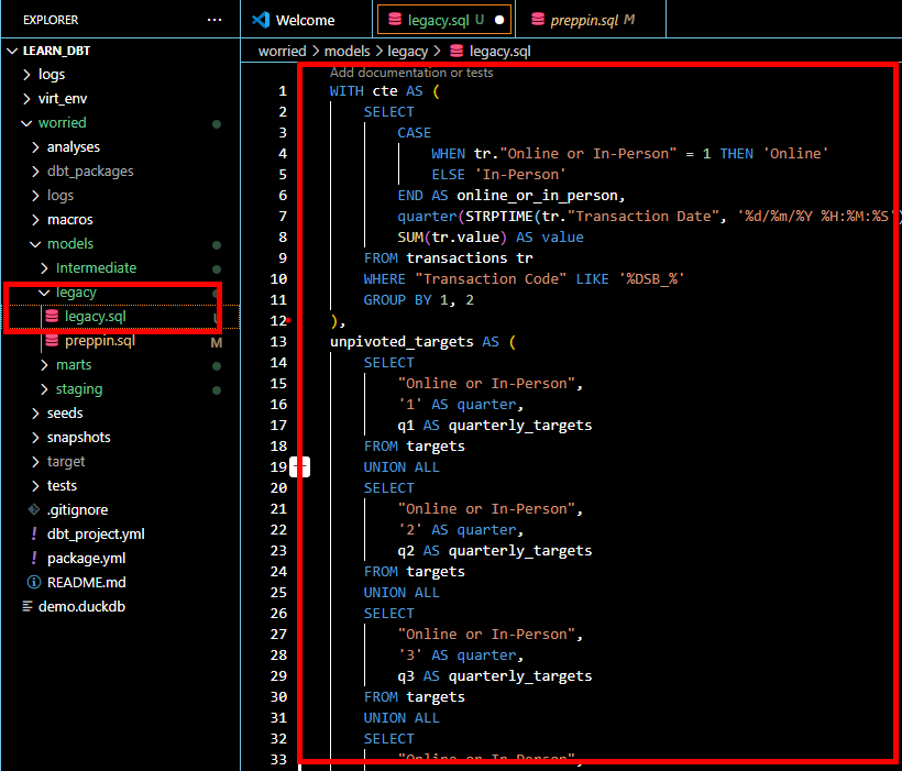
To illustrate modularity in dbt, lets have a look at this code (legacy script).

From the onset, we can observe how lengthy this script is and how tedious it could be moving up and down to digest the code if we had a script twice as long. For your information some scripts go as far 200 lines of code. In dbt, we can adopt modularity to break down these complex scripts into different models and enjoy its benefits.
To do this, we always need a refactoring method. For this example, lets hold on to our legacy script as our source of truth and place that in our legacy folder under models.
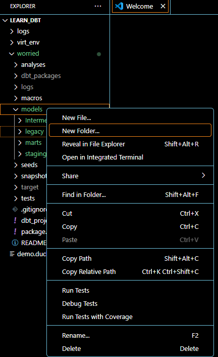
In the explorer pane under models, lets create a sub-layer called legacy by right clicking on models, select new folder and naming it legacy.
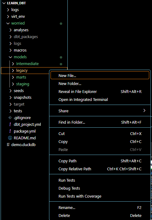
Create the legacy model by right clicking on the legacy folder, selecting new file, name it legacy.sql and paste the raw sql script in it.
Next is to create 3 more models using the same process employed above. Lets name these models "stg_dsb_transactions", "stg_quarterly_targets", and "fct_transactions_targets". We use the prefix stg_ and fct_ because classic dbt models could be layered into staging models, intermediate models, and fact tables. Staging models are usually connected to source data and takes care of basic transformations like column rename, metadata changes etc . Intermediate usually reference staging models and that is where our joins and aggregations are usually done. Fact models are where our final data preparations are done for further usage by analysts. Models in dbt are always defined as .sql files hence the need to create the file name using this syntax: model_name.sql. For the purpose of this example, we shall not make the intermediate model explicit.
To create these models, lets create 2 folders under model called staging and mart by right clicking on models, select new folder and name them accordingly.

Create the "fct_transactions_targets" under the marts folder by right clicking on the marts folder, selecting new file and naming it fct_transactions_targets.sql. Copy and paste the raw sql script form the legacy model into it for refactoring.
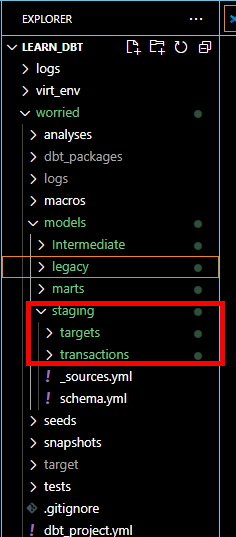
Under the staging folder, create two extra folders called transactions and targets to house "stg_dsb_transactions" and "stg_quarterly_targets" respectively.
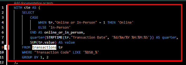
Under transactions folder, create the model and name it stg_dsb_transactions.sql . Go into fct_transactions_targets and trim out the aspect of the raw script needed for this model. Looking at the script, we can tell the first cte focuses on transactions so we can take that off but leaving out the aspect of aggregation.

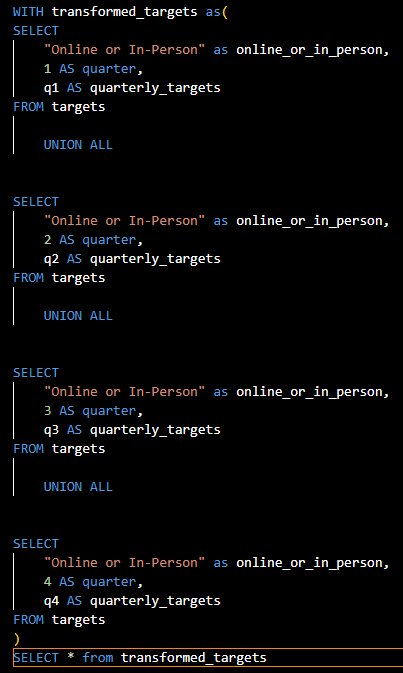
The second cte in the fct_transactions_targets looks at only targets so that portion can also be trimmed off into "stg_quarterly_targets" which will fall under the targets folder.
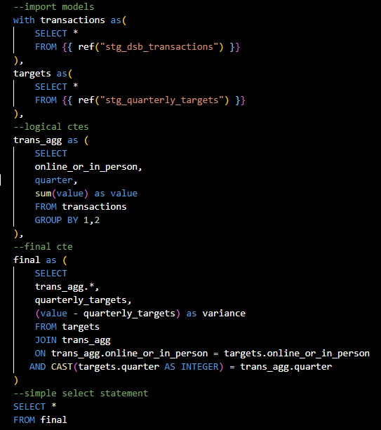
We can now go back to our "fct_transactions_targets" and reference our staging models using jinja template language for our import ctes, take care of aggregations in our logical cte and a final cte where we bring in all desired columns and make joins. Jinja uses this syntax: {{ macro(model_name) }}. For this example, we shall use the ref macro to call the relation to the specified models:
{{ ref("stg_dsb_transactions") }} , {{ref("stg_quarterly_targets") }} .
These 3 models should be saved using ctrl+s and run using dbt run. Upon running the models we shall observe that the staging models are created before the fact table since there is dependence from the fact table on the staging models which is made evident by the linage graph.
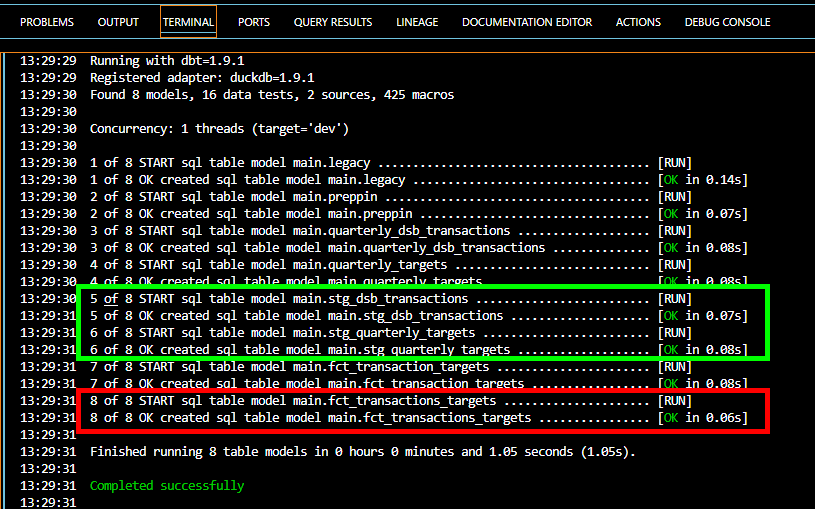
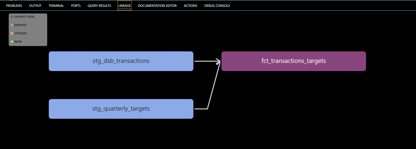
We can clearly distinguish how orderly the fact table is from the legacy script and how the dependencies are shown which grants us room to fish out errors easily when modelling.
Note: In this example, I have not implemented sources, run any tests or set materialization on my models. These will be done in my upcoming blogs for us to appreciate a deeper understanding of the importance of modularization in data transformation.
I hope this write up helped on your journey to learning dbt.