


A KNIME workflow is easy to follow: data moves from node to node, with each step representing a transformation. But what does the same workflow look like without the nodes? To find out, I took a simple KNIME workflow and rebuilt the same transformation logic three times in Microsoft Fabric: with Dataflow Gen2, SQL and Python.
The goal wasn't to find the best tool, but to see how the same data logic translates between three very different approaches.
All data used in this exercise is synthetic and does not represent real customer or company data.
Starting with KNIME
The original workflow uses transactional sales data and applies a series of familiar data preparation steps: aggregating customer data, selecting customer groups based on revenue and country, combining those groups and finally joining them back to the transactional data.
At a high level, the logic can be reduced to:
Load → Aggregate → Filter → Combine → Join → Sort
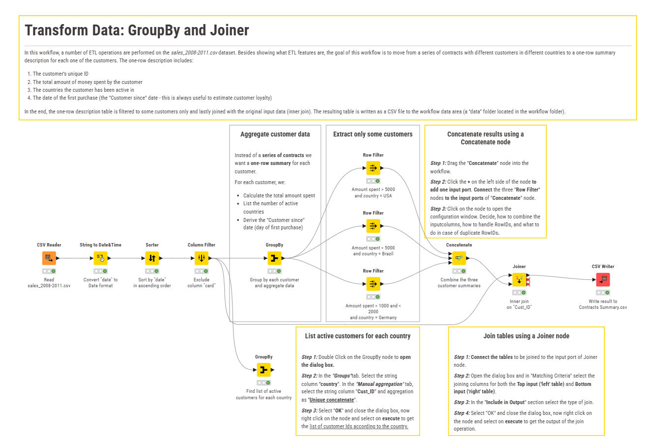
This made it a useful example for comparison. The transformations are simple enough that the focus stays on how each tool expresses the logic, rather than on complicated business rules.
1. Dataflow Gen2
I started with Dataflow Gen2, using Power Query to recreate the transformation.
Of the three approaches, this feels closest to working with KNIME. The transformation is still represented as a sequence of named steps, and each operation changes the result of the previous one.
The KNIME GroupBy, for example, becomes Table.Group in M. The three customer filters can be expressed with Table.SelectRows, their results combined with Table.Combine, and the final inner join performed with Table.NestedJoin.
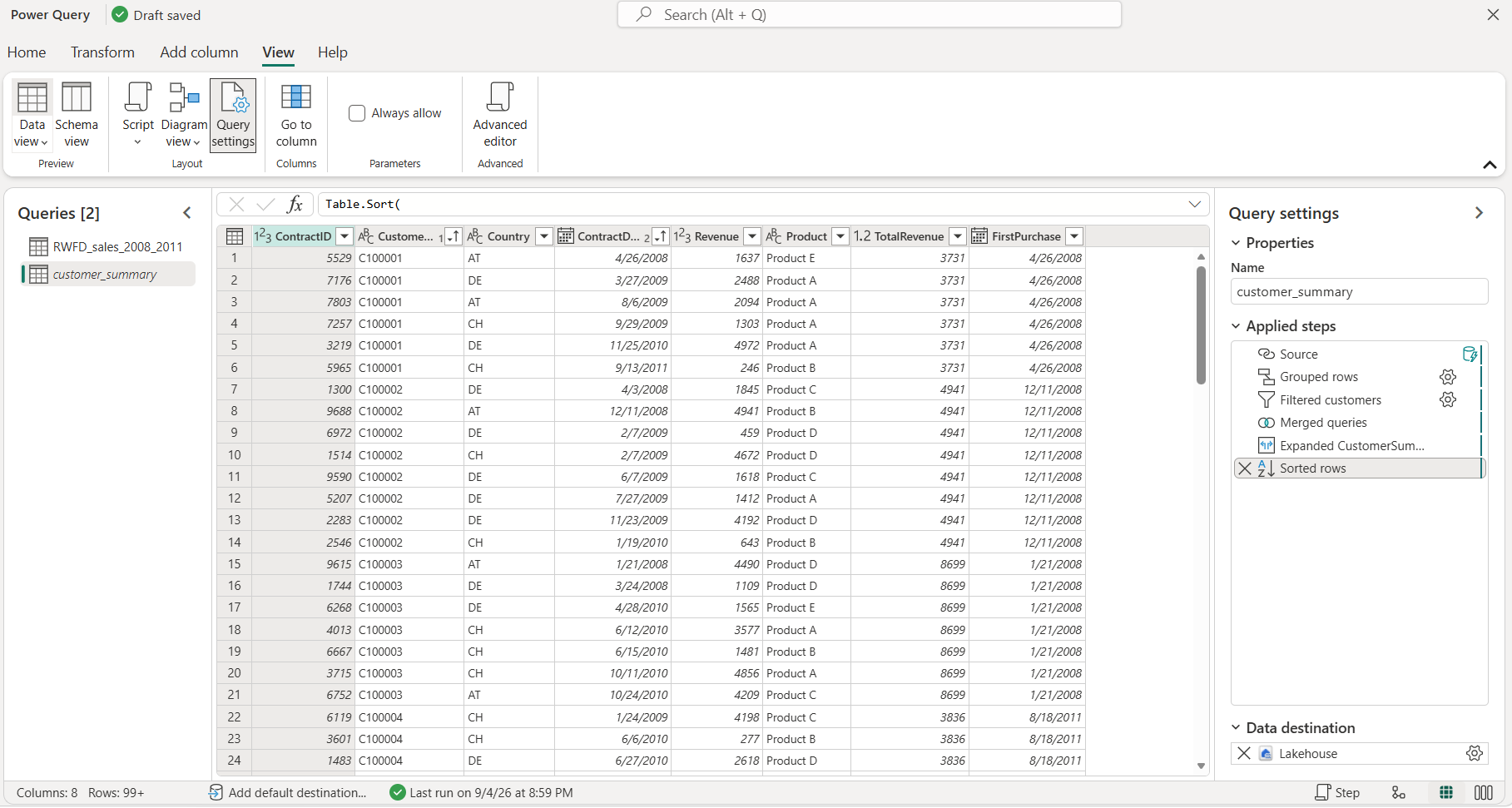
The interface is different, but the underlying way of moving through the transformation step by step remains quite familiar.
2. SQL
The same workflow looks very different in SQL.
Instead of moving through visual transformation steps, the logic is expressed declaratively. The customer aggregation becomes a GROUP BY, the three customer groups are selected using WHERE, UNION ALL takes the role of KNIME's Concatenate node, and an INNER JOIN connects the selected customers back to the transactional data.
WITH customer_summary AS (
    SELECT
        CustomerID,
        Country,
        SUM(Revenue) AS TotalRevenue,
        MIN(ContractDate) AS FirstPurchase
    FROM dbo.RWFD_sales_2008_2011
    GROUP BY
        CustomerID,
        Country
),

filtered_customers AS (

    SELECT *
    FROM customer_summary
    WHERE TotalRevenue > 30000
      AND Country = 'DE'

    UNION ALL

    SELECT *
    FROM customer_summary
    WHERE TotalRevenue < 10000
      AND Country = 'AT'

    UNION ALL

    SELECT *
    FROM customer_summary
    WHERE TotalRevenue BETWEEN 10000 AND 20000
      AND Country = 'CH'
)

SELECT
    s.*,
    f.TotalRevenue,
    f.FirstPurchase
FROM dbo.RWFD_sales_2008_2011 AS s
INNER JOIN filtered_customers AS f
    ON s.CustomerID = f.CustomerID
ORDER BY
    s.CustomerID,
    s.ContractDate;
What takes several separate nodes in KNIME can therefore be represented in one query.
3. Python
Finally, I implemented the same logic in Python with pandas.
Here the transformation becomes a sequence of operations on DataFrames. .groupby() creates the customer summary, Boolean conditions replace the Row Filter nodes, pd.concat() combines the customer groups and .merge() performs the final join.
import pandas as pd

sales = spark.sql("""
    SELECT *
    FROM dbo.RWFD_sales_2008_2011
""").toPandas()

customer_summary = (
    sales
    .groupby(["CustomerID", "Country"], as_index=False)
    .agg(
        TotalRevenue=("Revenue", "sum"),
        FirstPurchase=("ContractDate", "min")
    )
)

germany = customer_summary[
    (customer_summary["TotalRevenue"] > 30000) &
    (customer_summary["Country"] == "DE")
]

austria = customer_summary[
    (customer_summary["TotalRevenue"] < 10000) &
    (customer_summary["Country"] == "AT")
]

switzerland = customer_summary[
    (customer_summary["TotalRevenue"].between(10000, 20000)) &
    (customer_summary["Country"] == "CH")
]

filtered_customers = pd.concat(
    [germany, austria, switzerland],
    ignore_index=True
)

result = sales.merge(
    filtered_customers[
        ["CustomerID", "TotalRevenue", "FirstPurchase"]
    ],
    on="CustomerID",
    how="inner"
)

result = (
    result
    .sort_values(["CustomerID", "ContractDate"])
    .reset_index(drop=True)
)

display(result)
The workflow is again sequential, but unlike the visual Dataflow approach, every transformation is explicitly expressed in code.
Same Logic, Different Tools
Putting the three implementations next to each other made the similarities much easier to see.
| KNIME | Dataflow Gen2 | SQL | Python |
|---|---|---|---|
| GroupBy | Table.Group | GROUP BY | .groupby() |
| Row Filter | Table.SelectRows | WHERE | Boolean filtering |
| Concatenate | Table.Combine | UNION ALL | pd.concat() |
| Joiner | Table.NestedJoin | INNER JOIN | .merge() |
| Sorter | Table.Sort | ORDER BY | .sort_values() |
For this workflow, there is no meaningful winner.
The example is small enough that all three approaches work perfectly well. With more complex transformations, however, their different strengths become more relevant.
Dataflow Gen2 works particularly well for step-by-step data preparation and can also make transformations easier to understand and maintain in teams where not everyone is comfortable working with code. SQL is a natural fit for set-based operations such as joins and aggregations, while Python becomes especially useful when the logic is more algorithmic or iterative.
This also means that the approaches don't have to be mutually exclusive. The right choice depends not only on the transformation itself, but also on who needs to understand and maintain it.
What I Took Away
What I found most useful was seeing how directly the same operations translate between the different tools. Once I stopped thinking in terms of KNIME nodes and focused on what each step was actually doing to the data, the translation became fairly straightforward.
A GroupBy is still an aggregation, whether it is represented by a node, GROUP BY, Table.Group or .groupby(). The same applies to filtering, combining datasets and joining tables.
The tools express these operations differently, but the underlying transformation is essentially the same.