


What is Pacing?
Business targets are typically set on the quarterly or yearly level, but real-world data is generated much more granularly. Company executives will always be curious about how their business is doing, regardless of whether it happens to be the beginning, middle, or end of a given quarter.
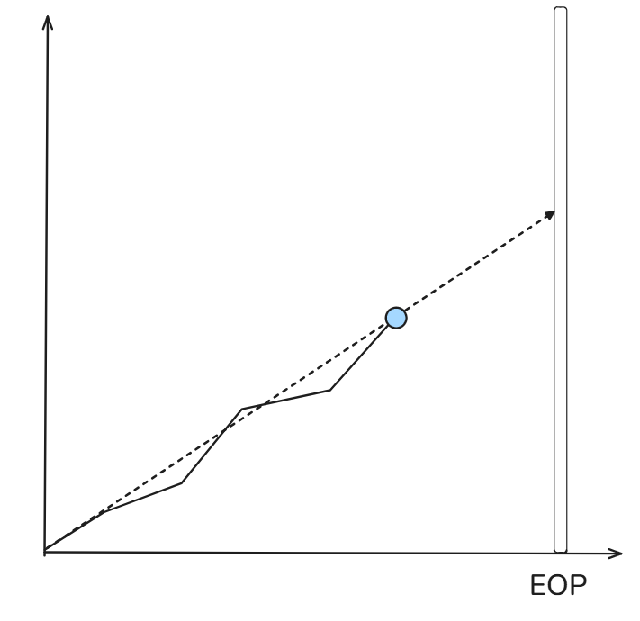
This problem is typically solved using linear pacing estimation, which is a (needlessly) fancy way of describing the mathematical process of estimating the slope to a given point in time, then extending that line to the end of the period. For example, if a company's yearly goal is $1,000,000 in sales and they have achieved $485,000 by the end of June, they are on pace for 2 X $485,000 = $970,000. The more general form of this process is multiplying the sales thus far by the reciprocal of the percentage of the period that has been completed. For the previous example, multiplying ($485,000) X (1 / (1/2)) = ($485,000) X (2) = $970,000. I primarily conceptualize this method graphically. In a visual representation, a line is drawn connecting the origin and the present moment, which is then continued to the end of the period. A quick mock-up of this idea is shown below:
When Linear Pacing Struggles...
Although this method is clean, it can lead to practical issues regarding sensitivity. For example, early in the period the multiplication factor tends to be extremely large, since it is the reciprocal of the progress through the period. In this situation, small changes can lead to extreme differences in projections. For example, on January 5th, a $1,000 change in sales would lead to a $70,000 change in total projection. This already differs from how an ideal pacing metric would intuitively work, but it can also lead to stakeholder dissatisfaction and overreaction. If it seems that sales is on pace but it is one order away from being portrayed as severely under pace, a stakeholder can end up misled and ultimately disappointed.
The statistical approach to this sort of challenge is usually to account for the amount of uncertainty that is present. The linear pacing model presumes a consistent amount of certainty throughout, but in actuality the beginning of the time period should be given less certainty and the end of the time period should be given more certainty. It might seem that those first 5 days of the year are under pace, but from a statistical perspective 5 days is far too small of a sample size to begin extrapolating out an entire year.
A Different Approach
When faced with this problem in the context of a Data School client project, I came up with a solution that is simple, modular, and incorporates the level of certainty that the linear method did not. The key change in framing is going from thinking of the projected total as a point estimate to considering it as a range. A range, commonly called a confidence interval in statistical applications (although that has more robust requirements that are not met here) is fundamentally made up of two pieces of information: a midpoint and a width. The midpoint was already there in linear pacing estimation, but the width will serve the role of confidence estimation.
You can find dozens of complex ways to forecast time series data to project a range estimate at a given endpoint, but I opted for a simpler approach. A final range has an upper bound and a lower bound, which I thought of as an aggressive goal and a conservative goal – language that is commonplace in a business setting already.
The aggressive goal is modeled as a percentage increase from the present trend. I imagined it being set at a 10% increase, but in practice this could be decided by a stakeholder or even left as a parameter for an end user to choose and possibly change. Similarly, the conservative goal is modeled as 10% below the current rate.
The key addition to this framework is starting the new slopes at the present moment. As soon as you switch from a constant rate to this range calculation, the size of the range starts to fan out, increasing in height the more time that passes since the switch.
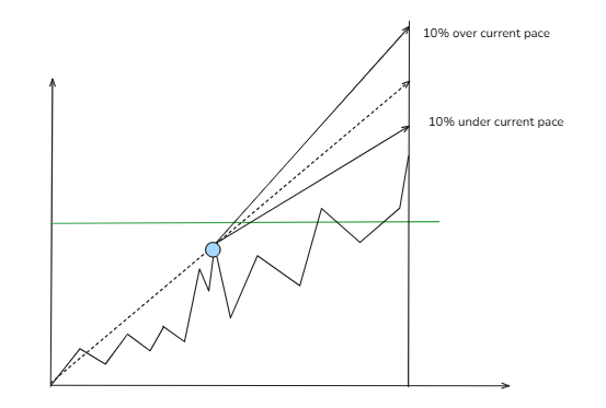
We can leverage this fanning behavior to create more uncertainty the further we are from the end of the period where the targets are set. If the fanning starts towards the end, there is not enough time for it to end up wide and you end up with a pretty confident, small estimated range for the projected total. Conversely, if the fanning starts at the beginning there is plenty of time for uncertainty to accumulate and the end of the period is reached with a massive range of possibilities. This behavior is illustrated in the image below:
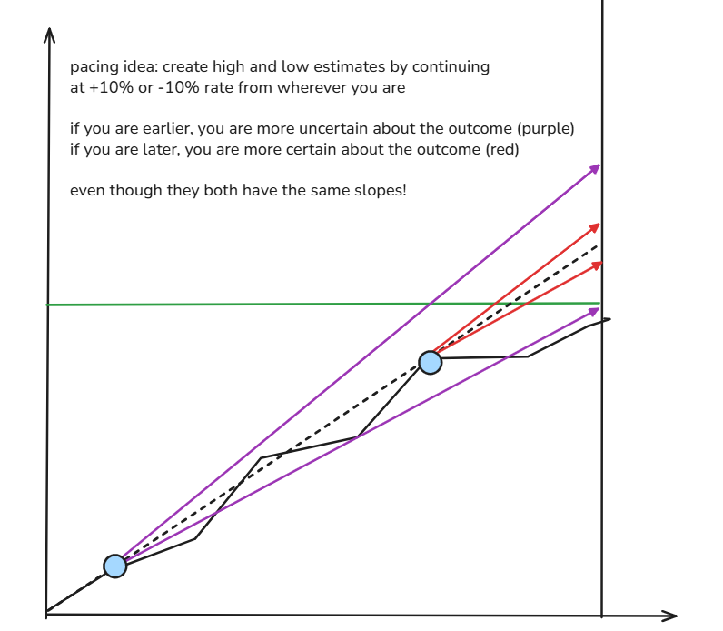
In the above example, there are two points that are found on the same rate line, but the one that occurs earlier accumulates more uncertainty, so its range includes values both above and below the green target line. For the later data point, the final range is tight enough to fully exclude any amounts below the target, making the user "confident" in the fact that the true end amount will be above the target.
That final example hints at the other advantage of outputting ranges instead of points: their placement relative to the target line can indicate the certainty of the projection. If the entire range is above the target line, even a conservative estimate would surpass the target, which is sufficient grounds to inform a stakeholder that the metric is on track to hit the target. If the whole range is below, even the most hopeful estimate does not reach the target, so the user can have higher certainty the target will not actually be reached. Alternatively, any range that includes the target amount suggests that it is too early to tell whether the target is going to be reached. This outcome ultimately addresses the prior issue of early-period sensitivity. In most situations, the reading for an early data point will be "too early to tell", which is far more appropriate and justified than overextrapolating minimal data.
In a future blog, I will implement this system in Tableau for the Sample - Superstore dataset, but I believe it is valuable to visualize the method in order to gain a better understanding before jumping into practical implementation.