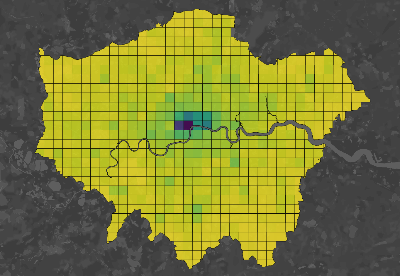
One possible function in Alteryx is using spatial information to create a grid over an area, and then input data into those squares to build a different kind of analysis. Through the use of spatial tools and a “Summarise” tool, this is a fairly easy and insightful way of breaking down data into more uniform shapes, particularly when considering areas that are not clearly defined.

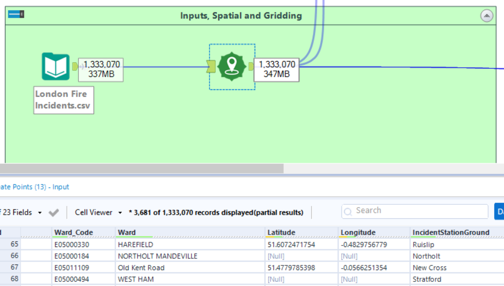
First, input your data. My first file contains information on reported fires in London: these come with latitude and longitude coordinates, essential when working with spatial. Having input this data, I then used the first spatial tool “Create Points”; through this, using the lat and long columns, you can create a point for each of the rows with coordinates. These will appear in your output columns under the title “Centroid”.

My second data input is using a shape file, containing London borough data. Being a shape file, this holds polygon information about the boroughs, viewable through a “Browse” tool connected to the input. Rather than being individual points (as with the first data input), these form distinct areas, hence the name ‘polygon’.
In order to create the grid, the next step requires the “Summarise” tool. Here, we can select the “SpatialObj” field (this is what Alteryx inputs polygons under), and in the spatial actions options, select ‘combine’. This creates one overarching area for London’s boroughs, rather than the distinct boroughs we had before. This is important, as it will allow the grids to be synced across boroughs, something necessary for quality of analysis.

The next tool is the “Make Grid” - simple enough to set up, this will create a grid pattern on your data, assigning grid names (and therefore polygons) for each square on the map. You can select the size of the grids (miles or kilometres), and also the specificity of the grid itself: depending on your setup, the grid will overlap edges, clip to the edges, or even become a single quadrilateral grid for the whole area.
Now it’s a case of joining these data inputs. Using the “Spatial Match” tool, the fire data (through the T [Target] input) will become data points integrated within the borough polygons (through the U [Universal] input), as the grid will form the basis for the data. The easiest way to understand these inputs is to think about them like darts: the U input is for the dartboard (the boroughs), whilst the T input signifies individual darts thrown at the board (the points themselves). The M input (Matched) will then output both the grid, and the overlaid points.

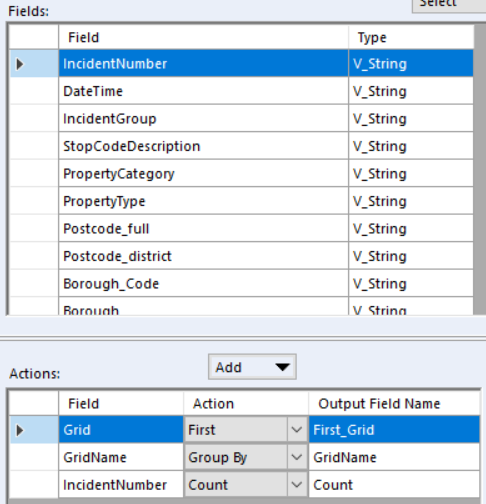
From this point, it’s a case of Summarising what you do and don’t want in your output: I kept it fairly simple and just brought in the Incident Number for analysis later on, but for Tableau, I also needed to bring out the Grid (I was able to pick ‘First’ as we only wanted one occasion of each grid square) and GridName (using ‘Group By’ as this impacted the data in the analysis per grid square). Use a “Browse” tool if you want to check just what you’re outputting at any point through this exercise.

Simply then output, and you’re done!

