Last week DS29 worked with Alteryx for the first time. In this blog I’m going to work through my thought process and the steps I used with various tools for my very first workflow. At the beginning of the day Robbin explained how each of the tools worked and thereafter provided us with the instructions and containers to assist us in the order of steps as to how we should approach the problem.
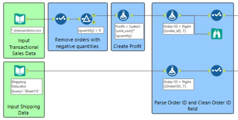
The basic containers we were provided with were as follows:

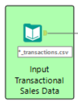
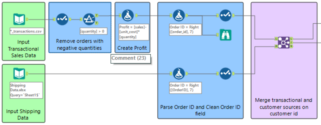
Step 1: Input the transactional sales data. This is done by dragging the ‘Input Data’ tool onto the workflow and selecting the file to be input. There were multiple transactional sales data in excel format to be input. We were taught about the incredible 'wildcard' which allows you to input multiple data files with one input tool. All file names had the ‘_transactions.csv’ in common and the wildcard was used as an * (asterisk) to substitute all subsequent characters that were different.
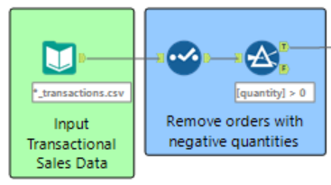
Step 2: Remove orders with negative quantities. I went about doing this by first using the ‘Select’ tool to change the columns in the data that were values from a ‘V-String’ type to ‘Double’. The help option on the configuration pane provides descriptions and examples for the different types of data as well as for any other description of tools and definitions. The ‘Double’ type is generally used as the default data type for decimal values.
Thereafter the ‘Filter’ tool was used. A custom filter was used to output the quantities that were greater than 0 out of the ‘T (True) anchor’ that meet the condition and the quantities that did not meet the conditions out of the ‘F (False) anchor’. The output True anchor is used for the following steps in the workflow as this data contains the positive values.
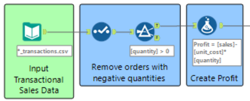
Step 3: Create profit. Using the ‘Formula’ tool a new column was created called Profit. This was done by creating a function that subtracted the multiplication of the unit cost and the quantity from the sales.
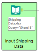
Step 4: Using a new input tool, the shipping data was imported into the workflow. Once the data has been input into the workflow, the ‘Browse’ tool can be used to show the data in table format in the data grid shown in the bottom white panel of the screen.
Step 5: Parse Order ID and Clean Order ID fields. I combined these two steps into one container. To parse the Order ID, the ‘Formula’ tool was used. A new column was created with a new Order ID which used the function Right(String, len). This function returns the last (len) characters of the string. In this case we needed the last 7 characters as these characters were identical for both sets of input data. The data was then cleaned using the ‘Select’ tool. The newly created Order ID column was replaced with the old one and the fields were renamed and formatted so they were easy to read and understand. This process was done for both of the input data.
Step 6: Merge transactional and customer sources on Customer ID. This was executed using the ‘Join’ tool. The transactional sales data was input through the ‘L input’ and the shipping data through the ‘R input’. The data was joined by two fields, namely the Order ID and the Product ID.
Step 7: Manage mismatched records as the data was not joined completely. Some records were output from the ‘L anchor’ which contains records from the L input that didn’t join to records from the R input. When investigating why this occurred, it was evident that some of the products had been ordered and collected instead of ordered and shipped. A formula was used to create columns for this data so that the ‘Ship Date’ was the ‘Order Date’ and the ‘Ship Mode’ was ‘Collected’. The output data from the Formula and the ‘R anchor’ data from the Join were stacked with the ‘Union’ tool. The Union tool input anchor accepts multiple inputs as indicated with the angle brackets. This unifies the two data streams. The configuration mode was set to the default setting to Auto configure by name. This stacks the data by the column name.

Step 8: Output file for use by business. I used the Auto Field tool which automatically changes the size of the field type to the smallest size possible. All fields were configured. The ‘Output’ tool is finally used to write the results of a workflow to supported file types or data sources. The first part is Write to File or Database dropdown where in this case the File was saved locally. The second part is to use the Options to select the file or database that you want to connect to. In this case the Alteryx database was used. The final workflow is depicted below.

