
Understanding Table Calculations
Table calculations are local calculations. Tableau queries your data source, pulls the aggregated data into your local machine, and then applies the calculation to what is visible in the view.
This is important as if your local machine is not powerful then Table Calculations can have a large impact on performance.
Another key property is that they depend entirely on what is in the visual, adding or removing dimensions from Rows, Columns, or the Marks card will change your results so be careful!
Creating a Table Calculation
When you right-click a measure we have two options for Table Calculations. We have a shortcut to apply some Quick Table Calculations alongside being able to select Add Table Calculation.
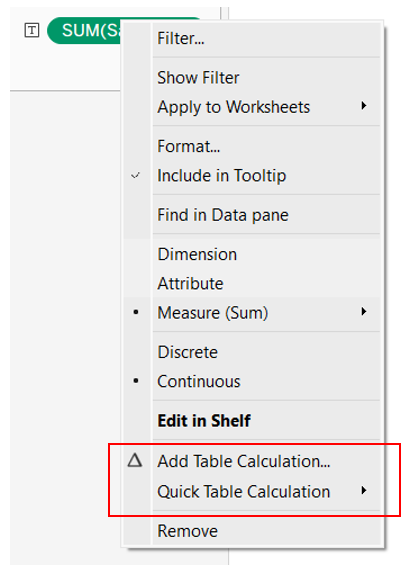
When we select Add Table Calculation we first select the Calculation Type.
Main Quick Table Calculations Explained
Here is how the primary calculation types operate mechanically within the configuration menu:
1. Running Total
- What it does: Progressively adds the current value to all previous values in the partition.
- Key Configuration Option: Running Selector. You can change the aggregation from Sum to Average, Minimum, or Maximum (e.g., a running maximum showing the highest peak achieved up to that point in time).
- You can also select to add a second secondary calculation. This allows you to perform a calculation on top of a calculation (e.g., calculate a Running Total of sales, and then apply a Percent of Total to that running aggregate).
2. Difference / Percent Difference
- What it does: Compares the current mark to another mark based on a relative position.
- Key Configuration Option: Relative to. * Previous (Default): Compares month-over-month or quarter-over-quarter.
- Next: Compares to the upcoming data point.
- First / Last: Compares everything back to the baseline anchor of your data set (e.g., comparing all subsequent years back to Year 1).
3. Percent of Total
- What it does: Calculates the current value divided by the sum of all values within the defined partition.
- Key Behaviour: If you choose Table (Down), the entire column adds up to 100%. If you choose Pane (Down), each individual pane adds up to 100%.
4. Rank
- What it does: Evaluates the values within the partition and assigns a numeric order (1, 2, 3...).
- Key Configuration Option: Rank Type:
- Competition - 1, 2, 2, 4
- Modified Competition - 1, 3, 3, 4
- Dense - 1, 2, 2, 3
- Unique - 1, 2, 3, 4
We then have Compute Using options.
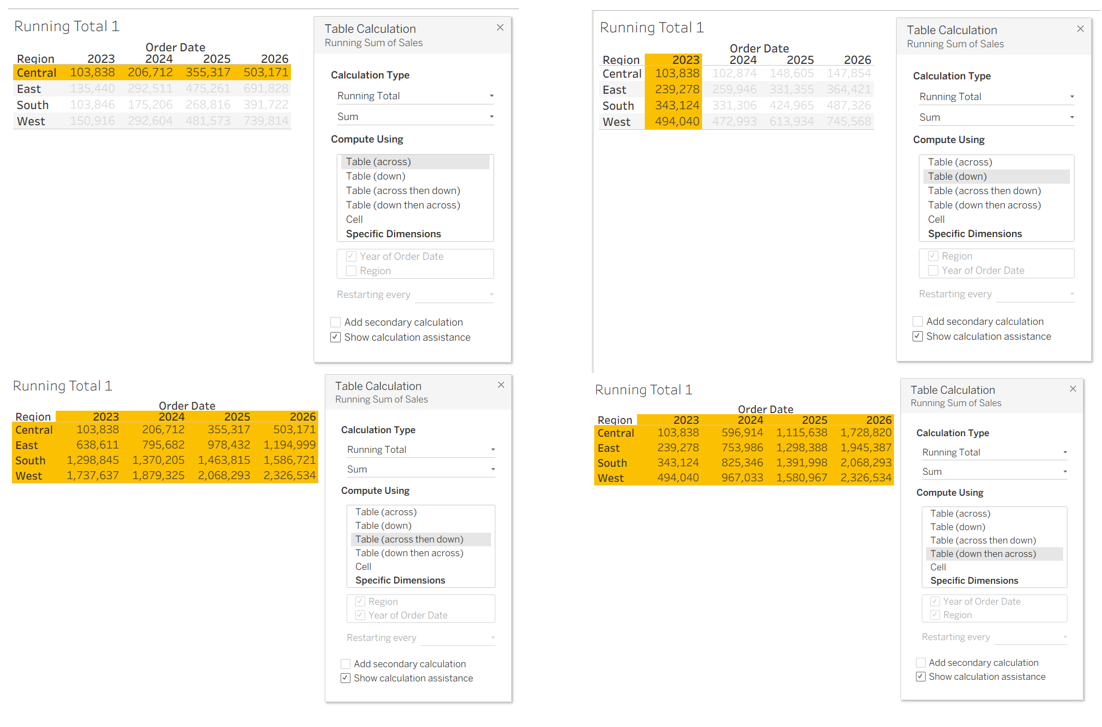
The "Compute Using" Options
- Table (Across): Moves horizontally across columns. It computes a value for each column and resets at the end of every row.
- Table (Down): Moves vertically down rows. It computes a value for each row and resets at the end of every column.
- Table (Across then Down): Moves across the entire row, then drops to the next row and continues the calculation.
- Table (Down then Across): Moves vertically down rows, then moves across to the next column and continues the calculation.
- Specific Dimensions: The most robust option. Checkboxes allow you to explicitly define which fields act as the Addressing (checked) and which act as the Partitioning (unchecked).
- Partitioning (Scope): Defines the boundaries. Which data points are grouped together? (Where does the calculation reset?)
- Addressing (Direction): Defines the direction. How does the calculation move through that group?
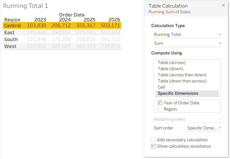
Here I've Partitioned By Region and Addressed By Year.
And once you've done all that you can identify your Table Calculations by the ∆ symbol next to your field: