Alteryx stats tools for beginners
This is part four of a five part series introducing the stats tools available in Alteryx explaining the tools and indicating when their use is appropriate.
- Clustering
- Data investigation
- Regression analysis
- Classification
- Time Series Analysis
Classification
In the previous post I looked at regression analysis of continuous variables; this post will address regression analysis of categorical (or discrete) variables, often termed classification.
Having discussed data investigation already in the previous two blog posts, I will dive straight into the process. It is relatively similar to the process for prediction of a continuous target variable, with a few important variations.
Data preparation
As I discussed in the previous post, we must investigate our data before we can begin modelling. We must decide how to handle any nulls in the data, understand the shape of the data, and investigate and possible remove any colliear variables within the data.
An additional aspect I will bring up here is that sometimes predictor variables may need normalisation. Normalisation is a technique by which we adjust the range of our predictor variables so that the difference between the maximum and minimum values is the same for all variables; the range of 0-1 is often used.
This is generally only necessary when there are categorical or binary predictor variables present. If these are in string format, they will need converting to numerical. With binary this is relatively simple, 1 for one value and 0 for the other. But what if there are three categorical variables, for example Red, Green and Blue. We could just assign a number to each: Red =1, Green = 2, Blue = 3; but does it make sense that Blue is twice as far away from Red as it is from Green? Is this ordering even correct? Should it go Red, Blue, Green?
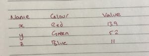
One way to handle this is to create a new column for each value of the categorical variable, in this case three: one for Red; one for Blue; and one for Green. Within these columns return a 1 if true and a 0 if false. This way you have removed arbitrary order from the colours and the arbitrary weighting of having a range of numbers.

This is where normalisation becomes a factor, if we have three columns with 1’s and 0’s, our sales data, which might range well into the millions, is dramatically more varied than the binary data. This may lead to uneven weighting of variables within the model. The get-around for this is to normalise all of the variables to range between 0-1.
The Information Lab’s Ben Moss has created a handy Alteryx normalisation macro.
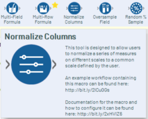
You can select the columns you want normalised and the scale of normalisation.
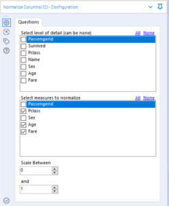
It is important that when using normalised variables to build a model, anything run through the model must also be normalised first, and any categorical variables that have been cross-tabbed and made binary but also be run through the model in the format.
The target variable can be in either a binary or a string categorical format.
Building a model
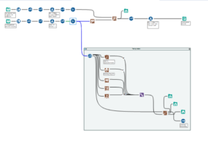
Sampling
As with regression modelling, we want to split our data into an estimation population and a verification population.
We will then run a number of models on our estimation data.
Choosing a model
As our target variable is discrete, the models we can use in Alteryx are:
- Boosted model
- Decision tree
- Forest model
- Logistic regression
- Naive Bayes classifier
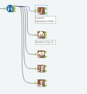
As before, I will run all of them, union the O outputs and run them through a model comparison, using the verification data to establish their efficacy.
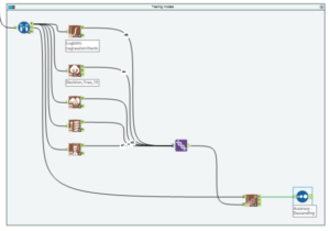
Comparing models
The model comparison will give each model a percentage score for over all accuracy, accuracy for each of the target variable outcomes, F1 score, and area under the curve (AUC). The closer to 1 that all of the values are the better.

The accuracy percentages are a simple measure of how many times the model got the right answer.
The F1 score is a function of precision and recall.

Precision is the number of true positives (model predicted true result correctly) the model predicted, divided by the total number of positives the model predicted – true and false positives (model predicted true result, but was incorrect).

Recall is the number of positives the model predicted correctly, divided by the total number of positive results in the data set.

The AUC refers to a graphical representation of the results, with true positives on the y axis (the model predicted a true result correctly), and false positives on the y axis (the model predicted a positive result, but it was actually negative).
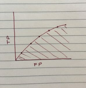
Which measure you give more weighting to depends largely on what your model is being used for. If you were creating an initial medical test, you would want there to be no false negatives, but false positives might not be such an issue; you don’t want any patients who are potentially ill to fall through the net, but you can afford to do further tests on patients who aren’t ill just to be safe. Conversely, if you have a test that is fairly cheap and easy, you may be less concerned with false negatives; you can always run the test again, such as with pregnancy or urine dipstick tests.
Model testing
Now that we have an idea of which model is best, we may wish to optimise that model by playing with excluding some variables or run it through the stepwise tool.
Once we are happy with the model, it is time to score it against some test data. As I mentioned above, it is important to normalise the test data if you did so for the training data. If you are going to be doing this process often, it might be useful to create a macro that normalises and cross-tabs any data that you are using to make the process easier for you and/or others.

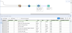
The results that come out of the model will look a little different from those which came out of the models for continuous target variables.

The results will give a probability for each of the possible outcomes for the categorical target variable, denoted by X_(result).
I then generally use a select tool to rename these columns to be ‘Probability of (result)’ and use a formula tool to change anything I converted to binary back again, or transpose anything I cross-tabbed before the modelling.
I hope this section has complimented the previous, and has been helpful. The final section on time series analysis can be found here.
