As a follow up to my random forest model blog, the next logical step is to explain the theory behind Alteryx’s gradient boosted model (GBM). Both models typically use an ensemble of decision trees to create a strong predictor. However, they differ in how they act at each stage of the ensemble. An ensemble is another way of saying multiple trees.

Before I go into further detail on the GBM, below is a chart that compares machine learning models, with GBM and random forest coming in first and second places respectively.

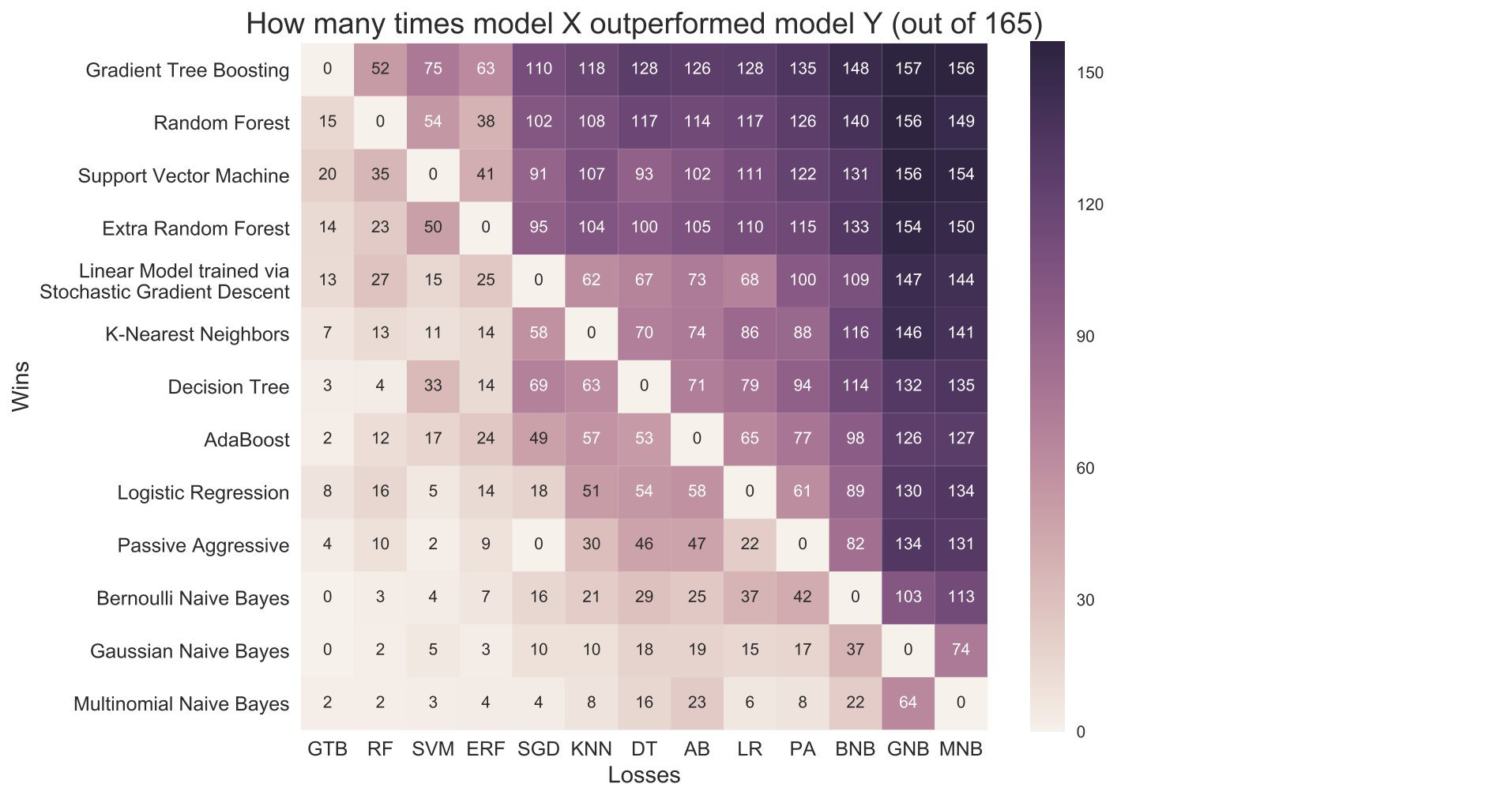
The reason behind GBM’s great performance against other models is how it creates a strong predictor by learning from the mistakes of its previous weaker predictions. A GBM model will assign weights to variables it predicted badly, in previous iterations, to help the new iteration adjust its algorithm accordingly. This is similar to human learning, as the model improves by focusing on improving on its weaknesses at each iteration.

The best way to explain this is visually in 4 steps, using images taken from – https://www.analyticsvidhya.com/blog/2015/11/quick-introduction-boosting-algorithms-machine-learning/.

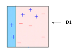
At stage 1 (D1), above, the model correctly categorised 7 of the 10 variables, thus leaving an error of .3. At this stage, it wrongly classified 3 +’s, so considering what I said earlier a weight will be assigned to these at the next iteration of the model. Below is the consequent result at stage 2, note that the wrongly classified +’s are larger and correctly classified variables are smaller to demonstrate the assigning of weights.

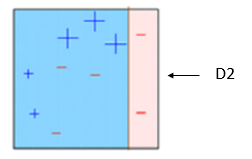
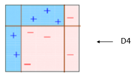
With the newly assigned weights, the model placed its categorising divide at the opposite side of the box. It once again got 3 variables wrong, this time the 3 –‘s in the middle. However, due to the change in weights to each variable, the error moves down almost a third to 0.21. The model will now move onto iteration 3 and reduce the weights on the correctly predicted variables, including the previously enlarged +’s, and add weight to the 3 –‘s that it got wrong. This now leaves the focus of the final stage on the +’s and –‘s that have been classified incorrectly once.

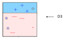
As expected the final iteration of the ensemble makes a division between the variables that had been wrongly classified once. It incorrectly distinguished 3 variables again, but once again the error is reduced, due to the weights, to .14.

Now, after 3 simple iterations, the power of the boosted model can be illustrated. To finish, the model will combine the previous 3 stages (weak predictors) to create a more powerful predictor. This is demonstrated in the image below where you can now see it can correctly classify all 10 variables.

With 4 simple images, the power of the boosted model is evident. When training different models to your data set it will often come out on top as unlike its opponents, it reduces error by learning from its own mistakes.