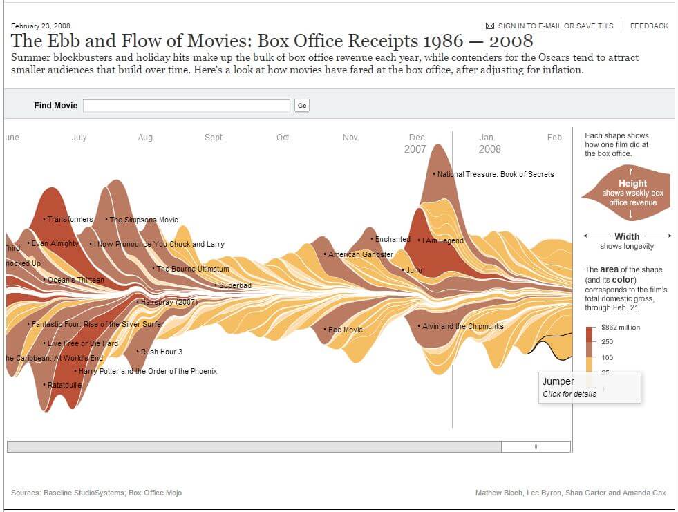
Stream graphs are wonderful for telling stories because they convey time in a very dynamic way. This famous New York Times piece exemplifies its execution – a measure that persists along a continuous time variable with some degree of interactivity. It’s fantastic for conveying running total but still allowing for the view to be anchored to a specific time period (like annual sales).

While not nearly as sophisticated as the NYT version, I wanted to share a tip about how you can create one of these graphs in Tableau. The concepts can be easily applied to more sophisticated vizzes. You can also download the workbook to follow along.

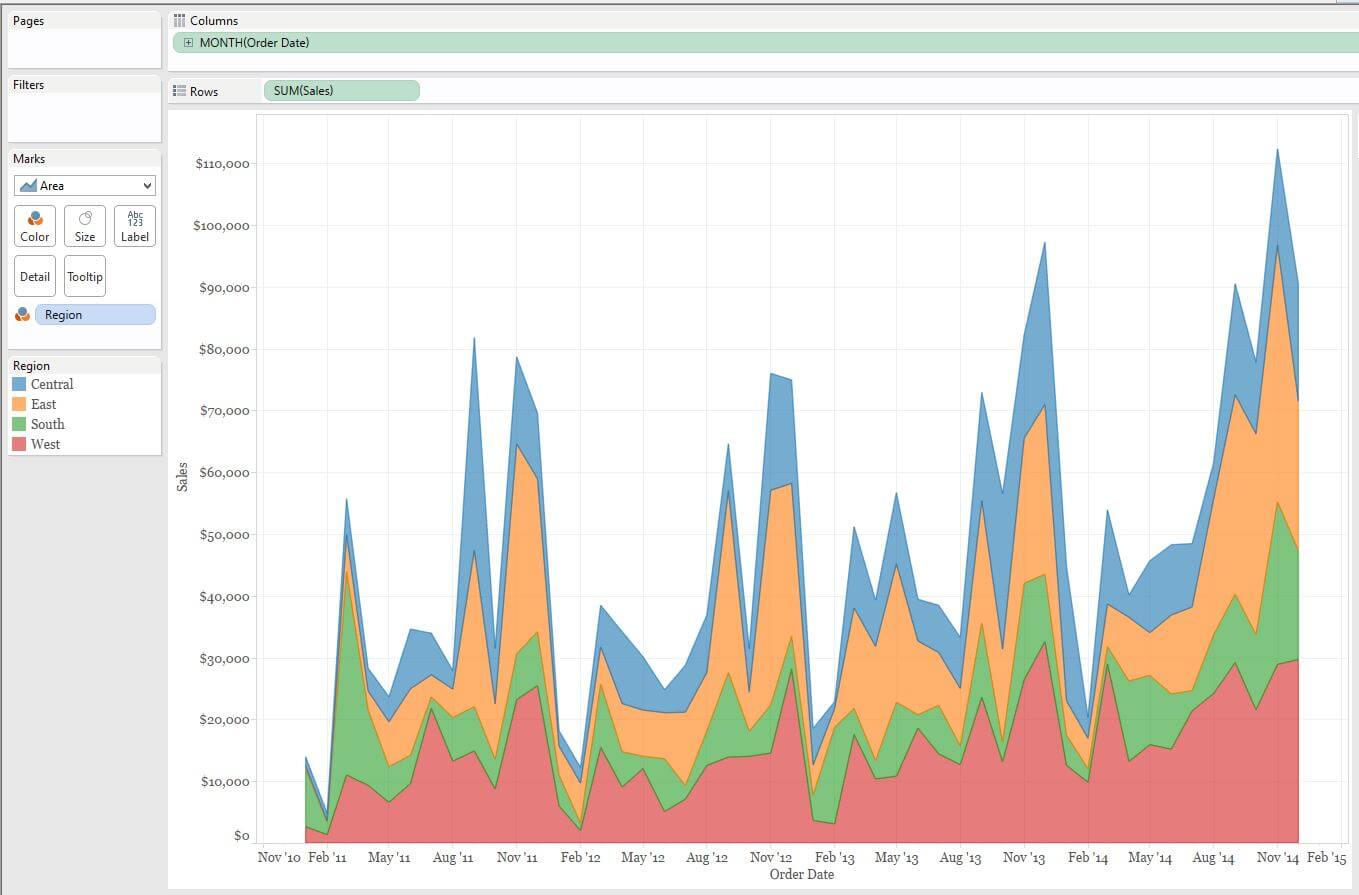
Step 1: Create an Area Chart with a Dimension on Color in the Marks Card. 

It’s helpful to create a view that’s pretty close to your desired end result. From there, it’s just figuring out the next steps. More of a mental thing I think 😀

Put “Date” on columns and “Sales” on rows. From there, add “Region” to color and set the marks card to “Area”.

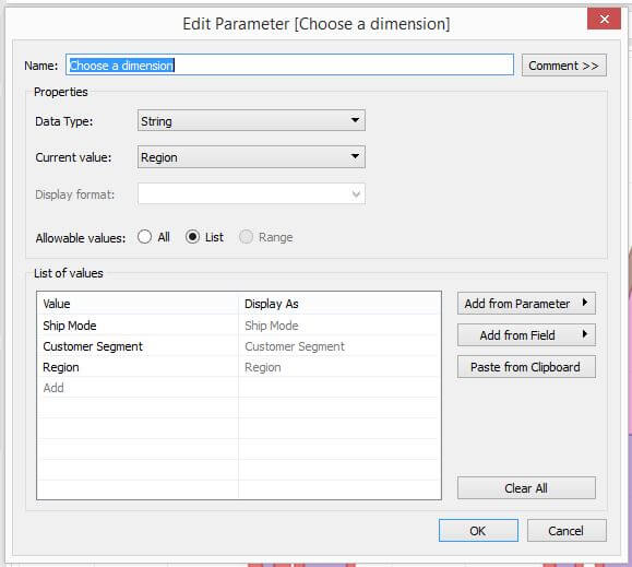
Step 2: Create a Dimensions Parameter

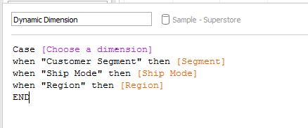
Pretty straight forward on the calculation for the parameter but here’s what I’ve built. Once you’ve got this pill set up, replace the region pill on the marks card with this new dynamic dimension parameter.

Here’s the initial parameter setup

Calculation to configure parameter actions

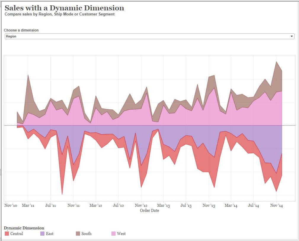
Step 3: Use Index() for the First Part of Sorting Sales into the Top/Bottom Side of the X Axis.

To get the stream graph’s iconic shape, we’ll have to bin the regions to show up either on top or below the x axis. We can do this by ranking the regions (our with our dynamic dimension pill on color) and creating a calculation that sorts the selected dimension to be above or below the x axis (essentially creating 2 bins  with 1 with positive values and 1 with negative values).

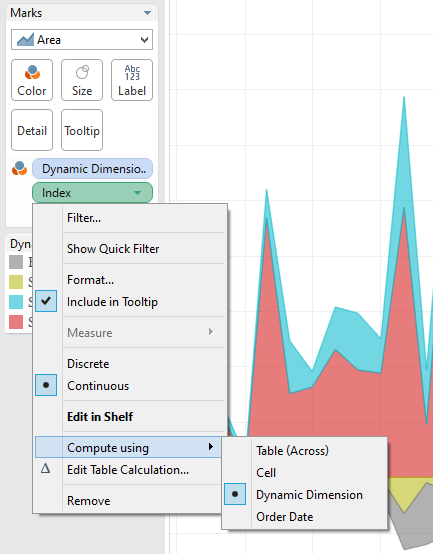
Firstly, we’ll rank the regions with the Index() function. Then we’ll add a table calculation set to “compute using” the parameter we’ve set up in Step 2.

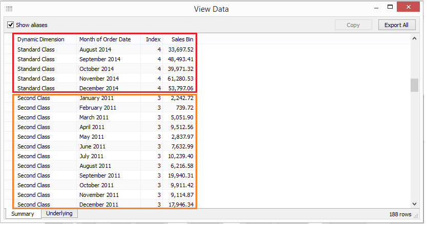
Here’s what the data is doing with the “compute using” – ranking the values within the “ship mode” dimension. We see that ‘Second Class’ was given an index of ‘3’ and Standard an index of ‘4’.

Step 4: Finish Sorting Sales into the Top/Bottom Side of the X Axis with an if Statement Binning Sales into Positive or Negative Values. 

In the calculation below, I’ve arbitrarily sorted index values 1 and 2  to show positive sales values (so the marks will appear above the x axis) and index values 3 and 4 to show negative values.

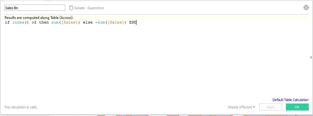
Replace your current sales pill with the one you’ve created here.

Then add a table calculation to this pill with compute using set to “dynamic dimension” or whatever else you’ve named your parameter controlled dimensions.

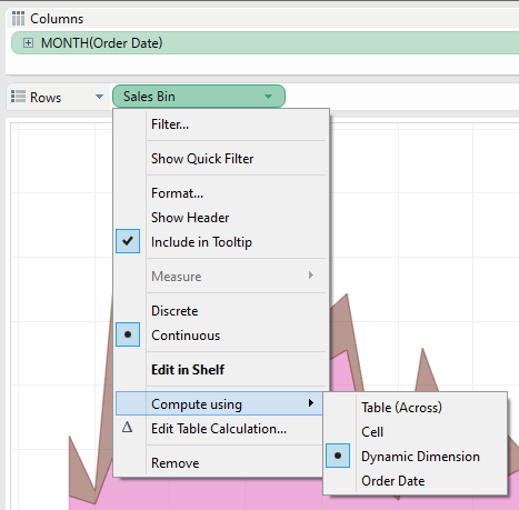
Voila! That’s it!