al

I recently came across this viz by Filippo Mastroianni of the late Stan Lee’s Marvel universe of superheroes and villains. Each data point is a character, which is sized by the number of appearances they made across the comic universe. What’s obviously striking about the viz is that the points are arranged to fit the shape of Stan Lee’s face. This got me thinking about how to prepare data for this kind of plotting in a Tableau viz, so I decided to give it a crack and blog about it.

In theory it’s quite easy to understand. The original image of Stan Lee’s face would likely be a two-dimensional matrix (2D: rows and columns) of binary values (e.g. 0’s and 1’s). Let’s say that 0’s refer to black pixels and 1’s refer to white. The black pixels of the image that are occupied by Stan Lee’s face would take the value of 0, and this is where you would plot your data in Tableau. The bits not occupied by Stan Lee’s face would be assigned 1. These would be the background points, where you don’t plot any data. Another name for this type of image is a 1-bit bitmap image.

If you are new to the idea of bitmap images, it’s good to think about very simple examples. Let’s take a ‘+’ sign as a demonstration. Here’s how you could draw a ‘+’ sign on a 1-bit bitmap:

If we wanted to plot data in the shape of this ‘+’ sign in Tableau, we would require two columns in our dataset that hold the X and Y coordinates of the 0’s. This is similar to the way that we require the latitude and longitude coordinates for plotting on a map of the world. Going back to our example, the coordinates of the 0 in the top row of our ‘+’ sign bitmap would be x=4, y=5.

Like I said, it’s easy in theory. But in practice, we’re going to hit some walls in terms of preparing our template image, such as:

• The image has more than two dimensions (think RGB levels)!
• The image has WAY more data points than the dataset I want to plot on it!
• How do I get the coordinates for the bits I want to plot on?!

I’m going to demonstrate how to use some relatively simple R code to prepare the image template and smash through those walls. If Alteryx is your thing, you can work with this code in Alteryx’s R Tool to achieve the same result.

1. Choosing a template image

The first step is to select the image that you’re eventually going to plot your data on in Tableau. In this exercise I’m going to plot some data about UFO sightings in the UK on an extremely simple clipart image of a flying saucer. This image will be easy to work with for a few reasons:

• It’s already black and white, so it will be easy to determine the 0’s and 1’s in the bitmap.
• There is clear separation between the background and foreground of the image. In images with different levels of colour and shading, it will be much more difficult to separate these out, and your image will probably require some extra processing before loading it into R. If you want to use a more complex image (like somebody’s face), it would be optimal to first turn it into a black and white stencil, like this image.
• The image has more black pixels than I have data points. In my dataset, I have 1905 UFO sightings that I want to plot. Later, you’ll see why it’s important to have plenty more pixels (especially black pixels) in the image than points in your dataset. That said, refrain from using huge images or your code will run very slowly.

2. Processing the image with R

Okay, try not to run for the hills at this point if you’ve never seen R code before! The code will be very adaptable, so you should be able to use it with simple binary images, regardless of whether you understand every line of code. I won’t go over the installation and setup of R here but there are plenty of resources online to help get you started. Here we go.

First, we’re going to need some additional R packages to load and process the image, namely the ‘magick’ and ‘OpenImageR’ packages.

install.packages("magick")
library(magick)
install.packages("OpenImageR")
library(OpenImageR)

Next, provide magick’s image_read() function with the URL to your image, and save it to a variable (I’ve named that variable ‘img’ in my example).

img = # Load image
image_read('https://i.etsystatic.com/7434544/d/il/ef2c1a/839898578/il_340x270.839898578_dfto.jpg?version=0')

We now have the image stored in ‘img’, which is of ‘magick-image’ class (specific to the magick package). We want to get to the pixel values of the raw image, so we’re going to convert the image to a bitmap like so:

# Convert to bitmap/matrix
img = as.numeric(img[[1]])

By investigating the dimensions of our bitmap ‘img’ using the dim() function, we can see that img is a 2D matrix of size 340 x 270 x 3.

dim(img)
[1] 340 270 3 

The first two dimensions refer to the number of pixels along the columns and rows of the image. The mysterious third dimension has 3 levels, which (spoiler!) refer to the RGB channels of the image. So, in this image file we have three 340 x 270 matrices, each corresponding to the red, green, and blue colour channel of the image.

Because our image is black and white, we don’t need this colour dimension, so we can just pull one of them out and work with that:

# Keep only one of the RGB channels
img = img[,,1] 

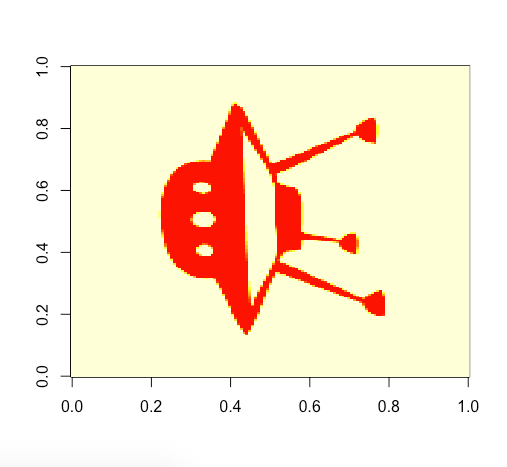
We can check how the image is looking using the image() function.

# Check image
image(img) 

It’s flipped it on it’s side for some reason, but we can sort that out later. R is also plotting it in red with a kind of yellow background, but that doesn’t really matter as long as we have a bitmap of 0’s and 1’s, so let’s move on.

3. Downsampling the image to a specified number of target pixels

This is where the magic happens. Not going to lie, I got very excited when this worked for the first time.

Let’s check how many 0’s we have in our image to potentially host our data points in Tableau.

# Count number of 0's
n_zeros = length(img[img == 0])
n_zeros

[1] 7445

7445. Way more than our dataset of 1905 UFO sightings.

So how do we deal with this discrepancy? The method I’m proposing is to downsample the image until there are only 1905 black pixels left. By downsample, I mean reduce the quality/resolution of the image, so it becomes more ‘pixelated’. Think about the picture quality of the first smartphone you ever bought. We’re taking the image back to the early noughties until it fits our dataset.

Here’s the downsampling code, followed by an explanation.

# Predefine number of viz coordinates/datapoints
targetPixels = 1905

# Downsample image to target number of 0's
for (i in seq(1,1000,0.0001)){
  
  img2 = down_sample_image(img, i)
  n_zeros2 = length(img2[img2 == 0])

  if (n_zeros2 == targetPixels){
    break
  } 
  
}

First, we predefine the number of 0’s that we want to end up with after downsampling (in our case 1905) and store it in a variable called ‘targetPixels’. The package ‘OpenImageR’ that we already loaded contains a function called down_sample_image() that we will use to (you guessed it..) downsample the image. This function takes two arguments – the input data (our image: ‘img’) and a downsampling factor. The downsampling factor is a numeric value that describes the degree of downsampling we apply to the image. A factor of 1 will cause the image to remain the same; a factor of 2 will reduce the number of pixels by half; a factor of 10 will reduce the pixels to a tenth of the original size, and so on. Our problem is that we don’t know what factor we need to downsample by to end up with our 1905 0’s.

The solution is to iteratively run the down_sample_image() function on our image file, and increase the downsampling factor by very small increments. In R we place the function within a for loop that will iteratively run the function with a factor that increases from 1 to 1000 in tiny steps of 0.001 on each iteration. We count the number of black pixels in the image on each iteration, and check if they equal 1905. When that criterion has been satisfied, we break out of the loop. Our perfectly downsampled image is now stored in a variable called ‘img2’.

Let’s see what our early noughties smartphone version of the image looks like:

Looks about right! All that’s left to do is rotate it back and extract the coordinates of the 0’s into a new data frame.

# Rotate image
rotate <- function(x) t(apply(x, 2, rev))
img2 = rotate(img2)

# Extract matrix coordinates of 0's
coords = as.data.frame(which(img2 == 0, arr.ind=TRUE))
names(coords) = c("PixelX", "PixelY")

I’ve stored the X and Y coordinates in two columns, aptly named ‘PixelX’ and ‘PixelY’ in a data frame called ‘coords’. You can output the data frame to a .csv file using the write.csv() function, and append it to your original dataset before loading it into Tableau for vizzing.

4. Plot the data to the coordinates in Tableau

Load the data into Tableau. Drop the PixelX pill on the Columns shelf, and PixelY pill on the Rows shelf. You should have some variable in the data that acts a unique identifier for each record in the data – drop that on Detail… and voila!

After a bit of scrubbing and sizing by the duration of the UFO sighting:

The possibilities are sort of endless with this one in terms of formatting/grouping data. It’s not going to work for every dataset and it’s not at all useful for comparing values. But it does look damn good.