A correlation matrix is handy for summarising and visualising the strength of relationships between continuous variables. Essentially, a correlation matrix is a grid of values that quantify the association between every possible pair of variables that you want to investigate. More often than not, the correlation metric used in these instances is Pearson’s r (AKA the “Pearson product-moment correlation” – but nobody talks like that in real life), which measures the extent of the linear relationship between two continuous variables. Pearson’s r ranges from -1 (a perfect negative correlation) to 1 (a perfect positive correlation), with 0 indicating no association between the measures. There are alternatives to Pearson’s r that aim to measure non-linear relationships, but Pearson’s r is by far the most common. Alteryx people might recognise correlation matrices from the “association analysis” tool.

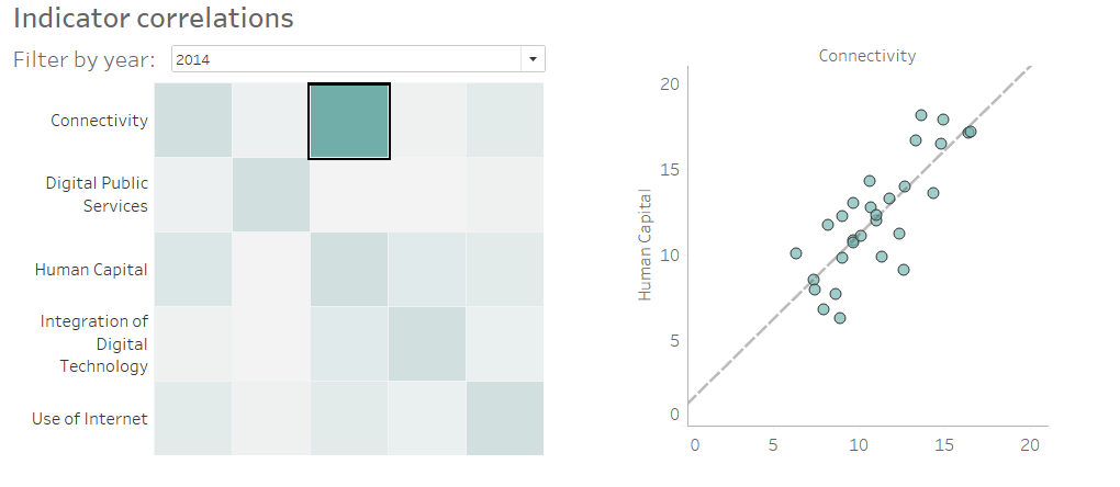
Here’s a correlation matrix I made in Tableau for Makeover Monday #5:

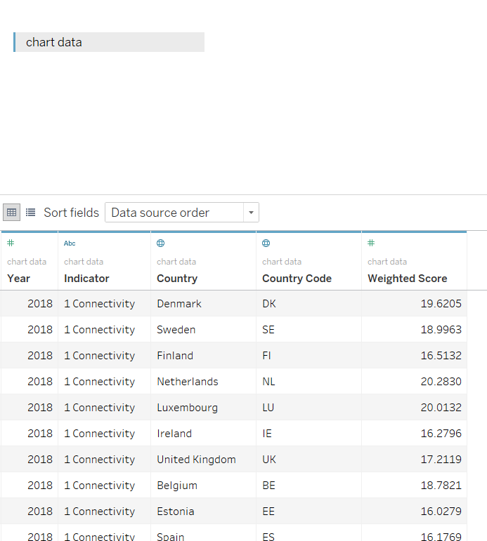
The diagonal values equal 1, because each measure has a perfect linear correlation with itself. The matrix is essentially mirrored from bottom left to top right as the measures are correlated in both directions. To illustrate how to make this with an example, I’ll use the DESI Makeover Monday dataset, which is available here. Firstly, connect to that dataset in Tableau.

Our objective is to visualise the correlation strengths between the Weighted Scores of each DESI Indicator. At first I thought the way to do this would be to put Indicator in the Rows and Columns shelf, and fill the cells with Pearson’s r computed in a calculated field. But no. Look what Tableau does:

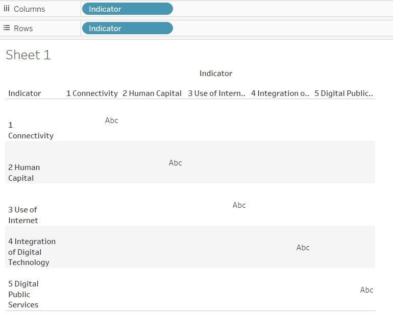
It only lets us fill the diagonals, which reflects the one-to-one mapping of each level of Indicator to itself. What we really want is to map each level of Indicator to every other level of Indicator. To achieve this, we need to duplicate the dataset and join them together.

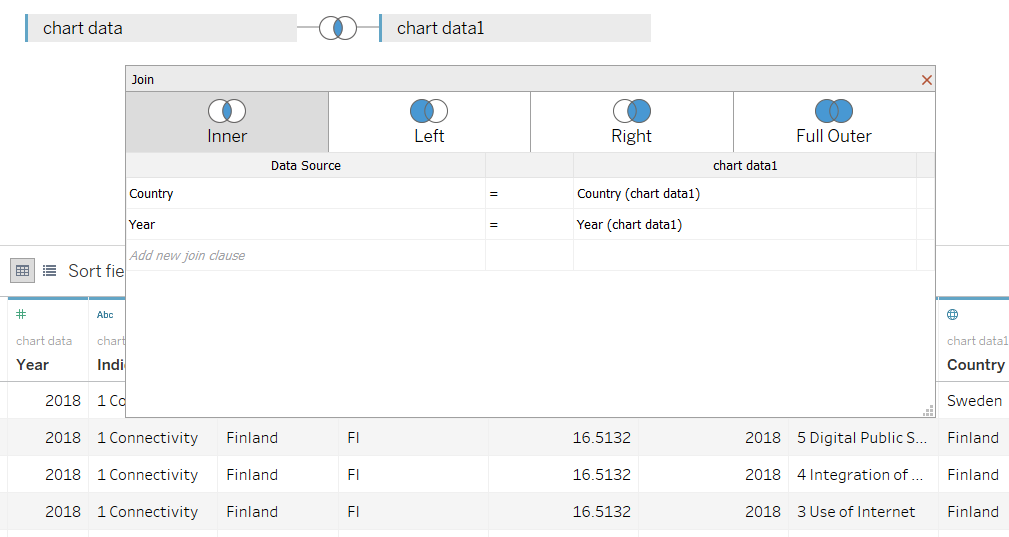
In the Data Source pane, join a second copy of the dataset back onto itself with an inner join. Now, we need to decide what fields to join on. Primarily, we want to join on the field that represents the highest granularity of our data: Country. Since we have data for the years 2014-2018, we can also join on year to calculate the correlations between Indicators for each year.

Next up we need to make a calculated field to compute the actual correlations. Tableau can compute Pearson’s r using the CORR() function, but a couple of LODs are necessary to construct the correct input values:

CORR(

{ FIXED [Indicator],[Country],[Year] : SUM( [Weighted Score])}

,

{ FIXED [Indicator (chart data1)],[Country (chart data1)],[Year (chart data1)] : SUM( [Weighted Score (chart data1)])}

)

At the core of this calculation we are correlating the original weighted scores ([Weighted Score]) with the joined weighted scores ([Weighted Score (chart data1)]) using the CORR() function. In addition, we’re fixing the scores across the Indicator, Year and Country dimension levels, which will be the dimensions in our view and filters.

The last step is to build the viz. Indicator, and our copy of Indicator go in the Rows and Columns shelf. Drop the Correlation calc on colour to fill the cells. If you want, you can enable the labels from the toolbar. Filter by Year, and you should get something like this:

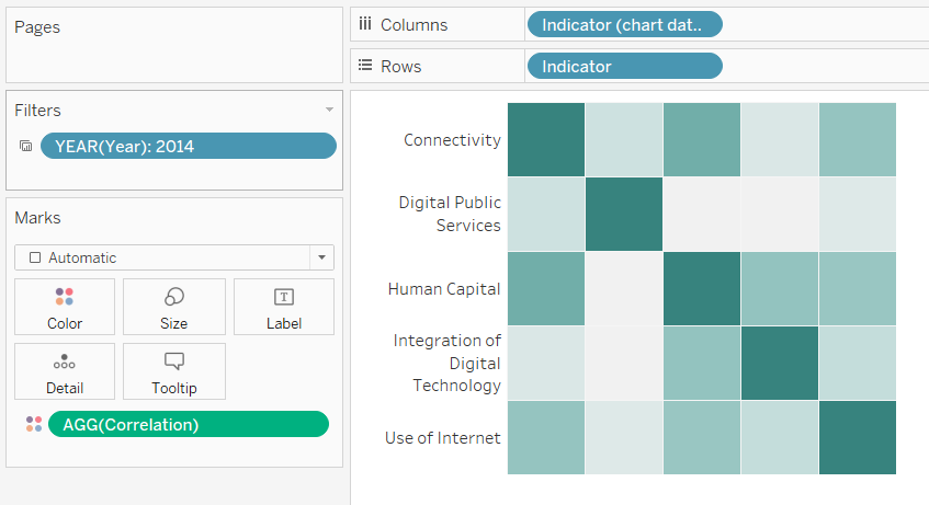
What I thought was really cool was the ability to use the cells of the correlation matrix to filter a scatter plot of those two indicators, which you could just as easily put in a tooltip.