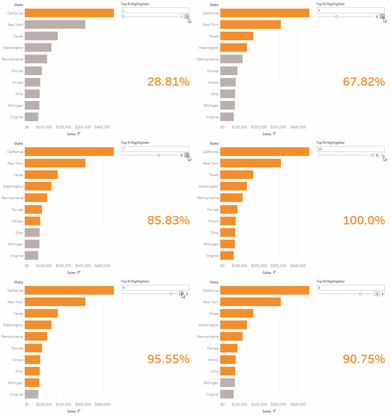
During the latest DS client project, I have implemented a functionality that allows highlighting a certain number of marks (in this example a Top-N bar chart) and dynamically displays the cumulative weight of these highlighted marks as a percentage of the total.
This gif should make easier to understand what I mean.

To do so we need to have a value sorted list
(in this example, a bar chart displaying the top 10 states by Sales from Sample-Superstore)

The first step is to build a parameter, this should be set-up as follows:
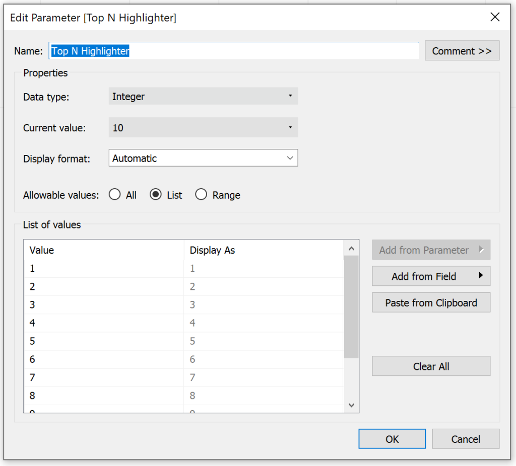
You can decide how many numbers to display. After creating the parameter [Top N Highlighter], right-click on it and show the Parameter Control.
Now create a calculated field using this formula
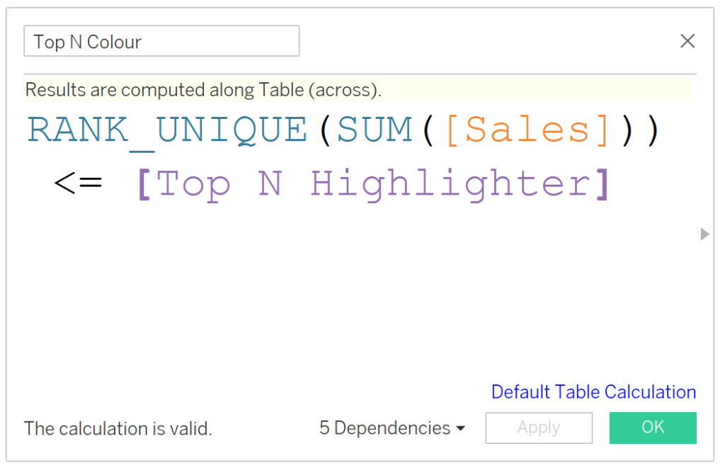
RANK_UNIQUE(SUM([Sales])) <= [Top N Highlighter]
Replace SUM(Sales) with your desired metric.
Drag this field to the marks colour shelf. You will be now able to use the Top N Highlighter parameter control to decide how many bars to highlight. You may want to change the colours to make the highlighted bar to stand out.
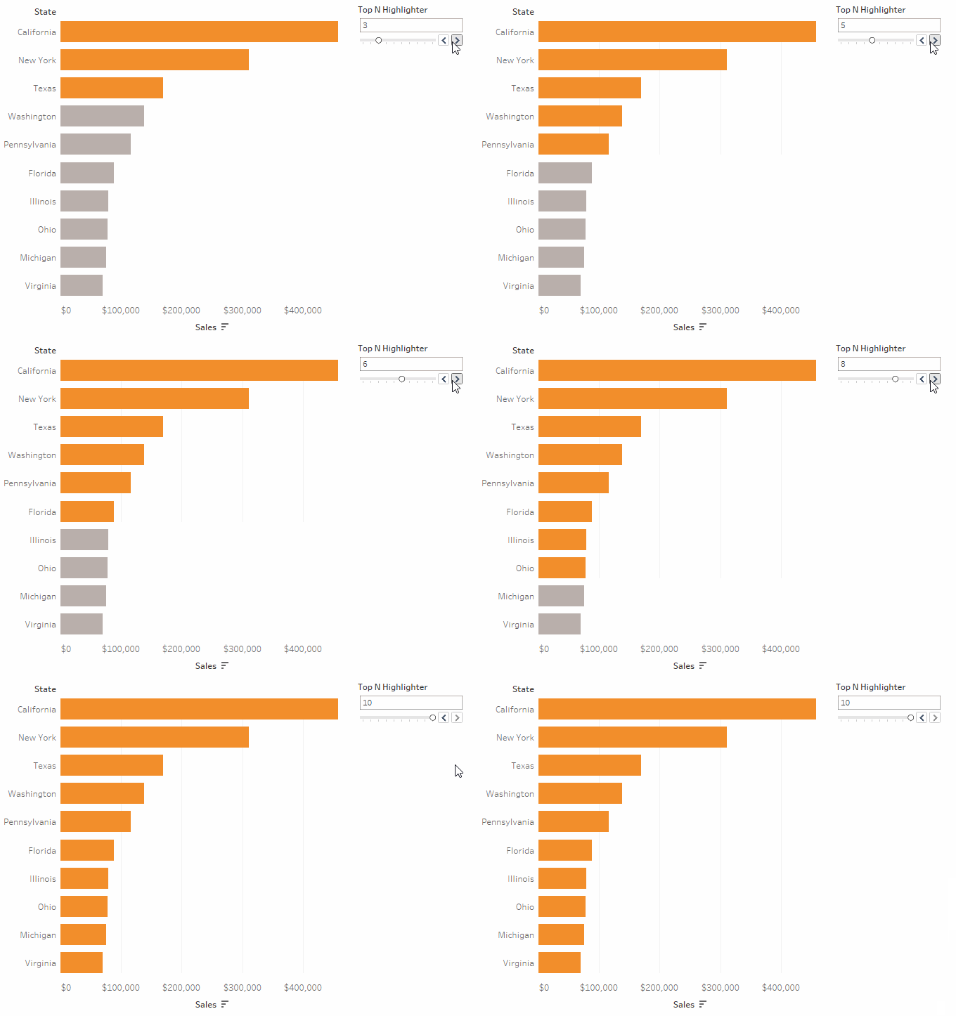
It is now time to implement the dynamic percent of total functionality.
To do so, first duplicate the bar chart sheet. From here:
- Move your measure SUM(Sales), to the text mark shelf.
- Add a Table calculation to the measure by right-clicking onto its pill.
- Configure the calculation as follows
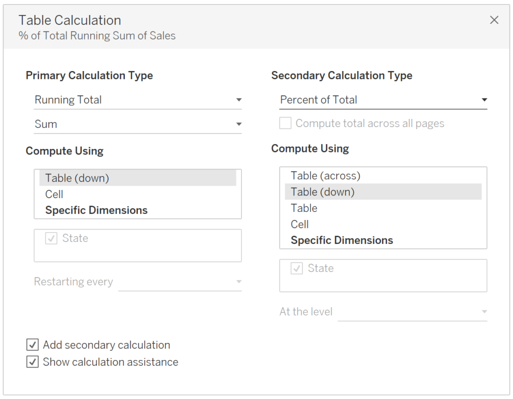
The primary Table Calc is computing a Running Total of Sales. The secondary one is computing the % of Total on the previously calculated Running Total.
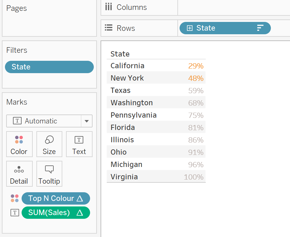
You can now notice that the percent of the total is cumulative, and it adds up to 100%.
Although we are only interested to display the highest number highlighted (which, in this example represents the cumulative % of the total of California and New York)
To achieve this we need to create a filter that would dynamically display only the latest highlighted value. To do so, create a calculated field using the following formula
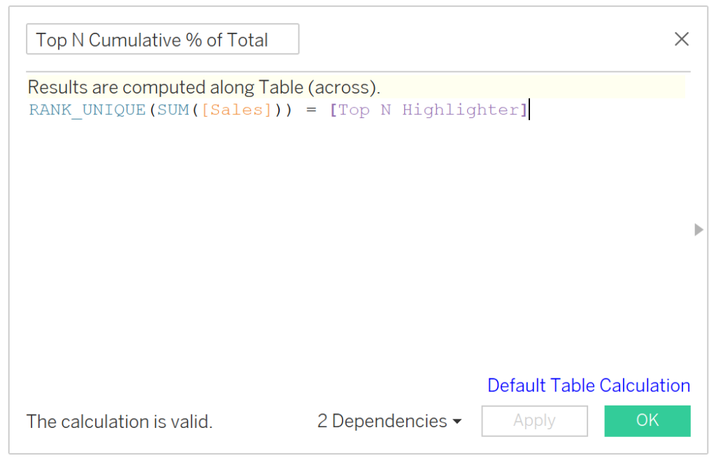
Drag this field to the Filters shelf and untick the ‘False’ option. This will now display only the latest percentage of our highlighted marks.
You can now format the view by hiding the category header and making the number bigger.
Now place both the sheets you have created onto a dashboard.
That’s it. Now you will be able to use the Top-N Highlighter to dynamically show the cumulative % of total.
